Guest post by Piers Forster, with comments from Jonathan Gregory & Ed Hawkins
Lewis & Crok have circulated a report, published by the Global Warming Policy Foundation (GWPF), criticising the assessment of equilibrium climate sensitivity (ECS) and transient climate response (TCR) in both the AR4 and AR5 IPCC assessment reports.
Climate sensitivity remains an uncertain quantity. Nevertheless, employing the best estimates suggested by Lewis & Crok, further and significant warming is still expected out to 2100, to around 3°C above pre-industrial climate, if we continue along a business-as-usual emissions scenario (RCP 8.5), with continued warming thereafter. However, there is evidence that the methods used by Lewis & Crok result in an underestimate of projected warming.
Lewis & Crok perform their own evaluation of climate sensitivity, placing more weight on studies using “observational data” than estimates of climate sensitivity based on climate model analysis. These studies, which employ techniques developed by us over a number of years (Gregory et al., 2002; Forster and Gregory, 2006; Gregory and Forster, 2008), have proven useful analysis techniques but, as discussed in the papers, are limited by their own set of assumptions and data issues, making them not necessarily more trustworthy than other techniques. Lewis & Crok suggest a lower estimate for climate sensitivity than the IPCC, but the IPCC did not make such a value judgment about the different methods of evaluating climate sensitivity.
Here we illustrate the effect of the data quality issues and assumptions made in these “observational” approaches and demonstrate that these methods do not necessarily produce more robust estimates of climate sensitivity.
Assumptions:
Lewis & Crok make much of the fact that our techniques employ “observational data” rather than a climate model. In fact, whilst they do not use complex dynamical climate models, they always use an underlying conceptual climate model. These underlying conceptual models make very crude assumptions and capture almost none of the physical complexity of either the real-world or more complex models.
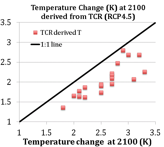
Varying the physics of these simple models such as ocean-depth, varying how data is analysed (e.g. regression methodologies), and varying how prior knowledge is factored into the overall assessment (Bayesian priors) all influences the resulting climate sensitivity (Forster and Gregory, 2006; Gregory and Forster, 2008). Particularly relevant, is our analysis in Forster et al. (2013) that confirms that the Gregory and Forster (2008) method employed in the Lewis & Crok report to make projections (by scaling TCR) leads to systematic underestimates of future temperature change (see Figure 1), especially for low emissions scenarios, as was already noted by Gregory and Forster (2008).
Observational data:
The “observational data” techniques often rely on short datasets with coverage and data quality issues (e.g. Forster and Gregory, 2006). These lead to wide uncertainty in climate sensitivity, making it hard to place a high degree of confidence in one best estimate.
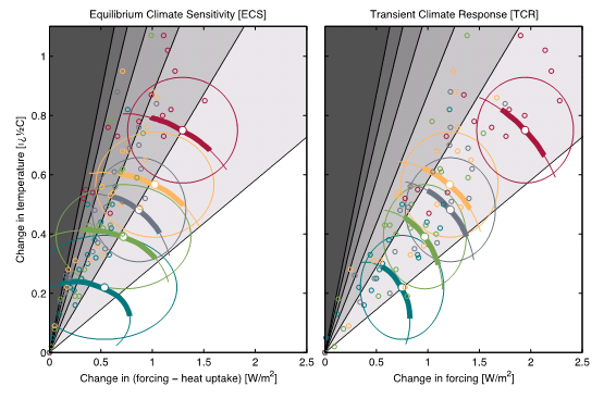
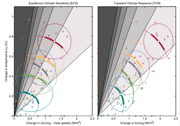
Particularly relevant for their analysis is the lack of global coverage in the observed HadCRUT4 surface temperature data record. Figure 2 compares the latest generation of CMIP5 models with the low climate sensitivity “observational data” analysis of Otto et al. (2013). In this figure the models have slightly higher climate sensitivity than suggested by the observations. However, in Figure 3, the CMIP5 models have been reanalysed using the same coverage as the surface temperature observations. In this figure, uncertainty ranges for both ECS and TCR are similar across model estimates and the observed estimates. This indicates that using HadCRUT4 to estimate climate sensitivity likely also results in a low bias.
Summary:
These are two reasons why the Lewis & Crok estimates of future warming may be biased low. Nevertheless, their methods indicate that we can expect a further 2.1°C of warming by 2081-2100 using the business-as-usual RCP 8.5 emissions scenario, much greater than the 0.8°C warming already witnessed.
References:
Forster and Gregory, 2006, J. Climate
Forster et al., 2013, J. Geophys. Res.
Gregory et al., 2002, J. Climate
Gregory and Forster, 2008, J. Geophys. Res.
Jones et al., 2013, J. Geophys. Res.
Otto et al., 2013, Nature Geoscience
One has to wonder what planet or universe you people write from.
This hastily written reply will be remembered as a sad tale of obfuscation. It does zero to resolve the lifelong problem of climate modeling, namely the inability to restrict the range of possibilities despite all the effort put in the last 35 years.
Lewis & Crok may have underestimated. That means they may have not. Their systematic problems are especially relevant for low emission scenarios. Then nobody believes there will be any lowering in emissions any time soon. Etc etc.
Ultimately, any idiot from the street can claim sensitivity is within the decades-old IPCC range. So instead of this futile and sterile PR attempts why don’t you do the right scientific thing and come up with something better than Lewis & Crok?
Maurizio – we have been doing the right scientific thing for decades by carefully sifting and assessing the science through the IPCC process, not making value judgements about which evidence to include and which to ignore.
It is great to see the GWPF accepting that business-as-usual means significant further warming is expected. Now we can move the debate to what to do about it.
cheers,
Ed.
Ed – stop circling the wagons. You weren’t there, decades ago to tell.
Back to basics. Lewis & Crok lower the old IPCC range. Furthermore, they make it narrower.
Your guest instead just argued that Lewis & Crok may be wrong, and we need stick to the old, wide, high IPCC range.
If your guest is right, climate modelling is pretty much useless and hopeless, apart from a vague feeling (utterably by “any idiot from the street…”) that things ought be warmer in the future (volcanic eruptions notwithstanding). That cannot be acceptable given all the money invested in it. This is policy-relevant stuff, not basic research.
The right thing to do then is to stop trying to answer science in five minutes on a Wednesday night and come back with a suitable riposte. Lewis & Crok challenged you modellers to provide a more useful range. Provide it, or disappear into policy oblivion.
ps further warming is expected. I am amazed you’d even think the GWPF has ever said otherwise. In what echo chamber have you been hiding for the past five years? The issue is how much, when by, at what rate, with what consequences. Thirty-five years of identical range of estimates provide zero clue about that.
“Sceptics” too often ignore the rather large accumulation of evidence from paleoclimate behaviour. For example, Rohling et al. (2012):
This issue does *not* simply hinge on GCMs-vs-“observational” estimates. However convenient it may be for contrarians to pretend that it does.
[snip – this is a scientific blog – please keep the comments scientific rather than political]
My comment was not political. Observational data should drive scientific models and not the inverse. My main point was that the last 4 IPCC reports must have had an effect to dissuade the 5th report authors from backtracking on previous dire predictions based on new flat temperature data.
Temperature has not been flat.
Ed Hawkins from his comment seems to me blissfully unaware of what to the educated layman at least appears to be the absolutely huge gap between current understanding (still pretty limited but making some progress) of climate sensitivity to CO2, and current understanding (infinitesimal by comparison) of natural as opposed to man-made drivers of global climate. Given the relative effort s put into understanding human influence (massive) and understanding natural change (tiny) this is probably unsurprising.
Hi Gillespie,
Not true – massive effort goes into understanding climate variability (e.g. see many pages on this blog) and natural forcings (e.g. read the IPCC report).
cheers,
Ed.
I’ve read way more peer-reviewed articles that deal with paleoclimate and climate changes outside of direct anthropogenic forcing than how the climate is necessarily changing now. Go here:
http://hetaylor.ca/enviro/gwnews.html#AWOGN20140316_Journals
and go through the archive. You’ll find many more articles on climate that make no mention of climate change but definitely have implications for it.
The mere fact that this response to Lewis and Crok’s paper has been hurriedly prepared makes me mightily suspicious that the Lewis Crock paper has hit a very raw nerve amongst the ‘consensus’ crew.
I have not yet had time to fully digest the Lewis/Crock paper yet since it has only just appeared but from first reading there seems little to argue with and a considerable amount to agree with. The fact that it is largely observationally based provides a credibility that is sadly lacking in the IPCC consensus claims of higher sensitivity.
John,
Lewis & Crok are part of the consensus. Their estimates are well within the IPCC range. And, yes, their method is observationally based, but it still uses a model, and as described in the post this approach is no panacea.
Ed.
More complex models do not imply greater predictive skill Mr Hawkins, in fact there is considerable evidence to suggest otherwise.
John, I agree. Simpler models are often easier to constrain
with data and have the virtue of being possible for a single person
To understand. Very well known in fluid dynamics.
So Foster is criticising his own method here? How very funny! About the only useful statement is “limited by their own set of assumptions and data issues, making them not necessarily more trustworthy than other techniques”.
Well quite! Everyone is basically guessing; some pessimistically and some optimistically. If you assume all warming from 1900 is manmade, and stick these assumptions in a model and then assume that the current unexpected plateau is not important then you will always see a high CO2 sensitivity. Alternatively if you assume, based on observations rather than the obviously inadequate climate models, that current warming is indistinguishable from the natural variation that went before 1950 – which is rather more plausible imo – then you get a CO2 sensitivity of zero degrees. These assumptions are otherwise known as Bayesian priors and the bias potential is obvious. One significant bias is that people whose livelihood depends on a high sensitivity will naturally choose the former interpretation because the latter one would put many of them out of a job. Another bias would be that if you disliked growth, cars and fossil fuel use in general then you will be more inclined to pin something on them. It has not escaped our attention that the previous global cooling scare was also blamed on fossil fuels – and wilder weather was also predicted for that cooler environemnet.
However, inherent in the more pessimistic assumptions is a corresponding very optimistic notion that it could be easy to move away from fossil fuels if we made them more expensive, therefore by our pessimistic will be doing future generations a big favour. Alas I hope it is now apparent that such is not the case: We are currently driving up the price of fuel by green taxes which causes suffering in the shorter term for no actual CO2 reduction and if the medium term causes blackouts and bankrupcy we know who to blame. Ironically the switch to shales gas, the ‘bete noir’ of environmentalists is doing more to reduce emissions than anything else. I urge you all to stop obscuring the fact that you are just making it all up – you do not know any more than any man in the street where the temperature is going and – you just pretend that you do.
No methods to derive TCR are perfect, or ever will be, including the “observational” estimates described here. The scientific thing to do is assess all the evidence from different methods, taking into account the caveats, assumptions, uncertainties from each and arrive at an overall assessment. This is what the IPCC does.
Ed.
You say that if you mask the CMIP5 models (presumably mostly the poles) so their coverage is the same as HadCRUT, the CS comes into line with the observational studies. You suggest that this indicates a cool bias in the observational studies. However, equally it could mean that the models run too hot at the poles. We already know that CMIP5 models run too hot (aerosols, the pause, Lewis/Crok Fig 3). We also note that global sea ice levels remain stubbornly around their long-term average level.
Should we not then conclude that the models are wrong?
HadCRUT4 lacks coverage in Africa, ME, Central Asia, Amazon Basin, areas of Australia *and* the poles (Cowtan & Way (2014) Coverage bias in the HadCRUT4 temperature series and its impact on recent temperature trends).
We might more readily conclude that:
– Observations are biased low
– There is no basis for the strong claim that “the models are wrong”
– Lewis’ aerosol estimate is too low (and you know this, because it has been brought to your attention by Richard Betts)
– Lewis’ estimates of ECS are biased low for these and other reasons
– You are not being sceptical enough
However, equally it could mean that the models run too hot at the poles.
There is data available for the Arctic, not included in the HadCRUT4 analysis, which indicates otherwise. Satellite data up to 85ºN, Arctic buoys and weather stations in the surrounding covered area. These data suggest rapid warming over the past thirty years and over the past century, in-line with model results.
The uncovered Antarctic region is less clear, and the models aren’t particularly consistent with each other there either.
In any case your argument is weak. We have CS estimates using observations without global coverage, and then comparisons to CMIP5 models with global coverage. Clearly this is not a like-for-like comparison so it makes sense to test how much of a difference it makes – the answer is apparently “quite a bit”. If we were to assume no information about trends in uncovered regions we can say it’s possible the models are running too hot in those areas, but it’s equally possible they’re not running hot enough – you didn’t appear to account for that possibility.
[Another relevant issue not often mentioned is that CMIP5 outputs used in these analyses are for global surface-air temperatures, whereas observations are LandSAT+OceanSST. This difference likely also produces a small cooling bias in observational trends compared to those from models.]
We already know that CMIP5 models run too hot
You seem to be engaging in a circular argument here. You “know” that CMIP5 models run hot, with the specific inference that they are too sensitive (do you mean all of them, some of them, on average?), therefore any evidence which indicates to the contrary must be wrong.
Lewis and Crok’s Figure 3 is subject to the same coverage and SST/SAT biases which have been mentioned here. Nevertheless, accounting for these biases still indicates the most recent 30-year trend is near the low end of the CMIP5 ensemble. Does that mean the models, on average, are oversensitive in a general sense? Not necessarily. Periods of around 30 years can be significantly influenced by natural internal variability (not mentioning potential forcing discrepancies at this point). This influence is apparent in the model ensemble, hence the trend variation depicted in Figure 3, albeit different models appear to produce markedly different amounts of interdecadal variance.
If you look at the bigger picture long term observed surface temperature changes appear to be clearly consistent with the model ensemble, although there is substantial variation in the latter (Note the labels indicating the steps taken to produce a like-for-like comparison, also the model data only goes up to the end of the historical run – 2005). From the same data time series for 30-year trends indicate a few occasions in the past where observed trends have gone outside the “prediction” envelope of the CMIP5 ensemble, both low and high, yet the centennial warming is still consistent.
“Periods of around 30 years can be significantly influenced by natural internal variability”.
Like, say, 1910-1940 and 1970-2000?
Too often, unspecified “natural internal variability” is invoked to explain away periods of less warming. An even-handed approach demands that natural internal variability be considered equally in periods of more warming.
Then why is GAT ~0.8C higher than it was in ~1850? Natural variability averages out over time.
BBD: “Then why is GAT ~0.8C higher than it was in ~1850? Natural variability averages out over time.”
First, I think you mean natural *unforced* variability.
Secondly, you can get shifts in operating points of complex systems, where the system shifts to a new stability point, and never moves back (until something external bangs on the system hard enough).
Even allowing this, over what time scale?
As long as you’re in the 1/f^n portion of the spectrum, it doesn’t average to zero…. this is the famous random walk pattern, where the observed variance increase with the duration of the observation period.
[Note this is not a superficial comment on the likelihood that the current warmer temperature are due to just natural variability, which I actually think is improbable.
Nor do I suggest that on sufficiently long time scales that the Earth’s system would resemble a random walk, or that temperature fluctuations would retain a 1/f^n spectrum form.]
Not necessarily (TSI) but I take your point. But like you, I don’t believe in a self-propelling climate system. Random walks in climate do not go very far before conservation of energy steps in.
“natural variability averages out over time”. Wrong. I don’t have much trouble accepting that natural internal variability is very likely to average out over time, but natural variability clearly does not average out over time. Certainly not over any meaningful timescale anyway. Otherwise there would not be ice ages, interglacials, etc, and we would not be expecting anything significant to happen in the next 5bn years.
Why is GAT ~0.8C higher than it was in ~1850? Possibly (probably?) for the same reason that it is almost certainly lower than 1,000, 2,000, 3,000 years ago : natural variability.
Unforced natural variability simply moves energy around within the climate system. It does not create energy. Therefore it cannot generate long-term trends and it averages out over time. This is not in dispute, btw, so you are on your own here.
Glacial cycles are orbitally forced, which is why Carrick added the qualifier *unforced* natural variability above. You are getting muddled up, but I have to take some of the blame for writing sloppily.
These claims are contradicted by the evidence. See eg.PAGES2K (2012):
The evidence suggests that the last decade is probably hotter than any time since the end of the Holocene Climatic Optimum ~6ka (Marcott et al. 2013). The HCO was orbitally forced, so there’s no mystery as to why it was warmer then. Nor is there any mystery as to why it is getting so warm now.
“However, equally it could mean that the models run too hot at the poles.”
Andy, that assertion would be sad if it weren’t so funny. In the real world, the models demonstrably run cold relative to the poles. Perhaps worse is that they can’t manage a transition from current to mid-Pliocene-like conditions (in equilibrium with *current* CO2 levels).
Ed,
That’s very interesting. I had wondered if this had ever been done as it seemed an obvious test. Has anyone done a comparison between an Otto et al. analysis using Cowtan & Way with the ECS model estimates with global coverage?
Not that I know of. My guess is that this would increase the estimates of TCR, but it would be interesting to find out. Maybe Piers could do it?!
Ed.
Great idea, I’ve been thinking we should do it with lots of datasets in fact including satellite data tropospheric temperatures and reanalyses. I was really surprised masking made so much difference, but, just as you say in your blog, adding a few years of data also makes a big difference, which really adds to the evidence that these techniques are not that robust
Just out of interest, does anyone have any comments about this result from Lewis (2013)
My understanding is that the first result is obtained using data from 1945-1998 (I think). This gives an ECS of 2-3.6K. Adding 6 years of unused model data (which I understand takes the time interval to 2001) changes this to 1.2-2.2K. That seems like a remarkable change given that it’s only an increase of about 12% in data. Wouldn’t one expect a method that estimates something like the ECS to be reasonably insensitive to relatively small changes in the time interval considered. Or, have I misunderstood what Lewis (2013) has done here.
I agree. This is potentially a problem with using the observational period to derive ECS. Maybe TCR, which is the most relevant quantity for projecting warming over the coming decades, is less sensitive?
Ed.
My understanding is that in Lewis (2013) the comparison is done with models that have different ECS, Aerosol forcings and ocean diffusivity. The method then determines which models produce the best fit to the observations. So – if I’ve got this right – Lewis (2013) cannot estimate the TCR because I don’t think that was one of the model variables. Of course, I guess each model should have a TCR value, but I can’t find any mention of this in Lewis (2013). Given that this is based (I think) on Pier’s earlier work, he could comment more knowledgeably than I can.
Apologies, I think I may have just confused Forest with Forster 🙂
The point of the Lewis 2013 study was to recalculate Forest et al 2006 using an objective prior rather than the uniform prior in ECS used by Forest. The shift in the long tail is due to that rather than up to date data.
In the report, Lewis/Crok note of the Otto et al study:
“In fact, best ECS estimates based on data for just the 1980s and just the 1990s are very similar to those based on data for 1970–2009, which demonstrates the robustness of the energy budget method.”
One should distinguish between Lewis (2013) and Otto et al. (2013). In Lewis (2013) the result when using the same time period as Forest et al. (2006) has quite a large overlap [2.1 – 8.9K compared to 2.0 – 3.6K]. Adding 6 years of new data, changes the ECS range to 1.0 – 2.2K. So, yes if you use the same time interval as Forest et al. (2006) you can reduce the uncertainty in the high end, but why would one not be concerned by the significant change in the estimate when adding only 6 years more data?
Your quote appears to be based on the Otto et al . work, not Lewis (2013). I agree that Energy budget constraints are quite useful, but I think many would argue that they do suffer from various issues related to regional variations in ocean heat uptake, uncertainties in aerosol forcing, missing coverage in the temperature datasets. If one assumes that the recent Cowtan & Way result has merit, then that would increase the ECS and TCR estimates from Otto et al. by a few tenths of a degree.
Having referred to the Lewis 2013 paper (a draft – struggling to find the final version) he says:
“We resolve these issues by employing only sfc and do diagnostics, revising these to use longer diagnostic periods, taking advantage of previously unused post 1995 model simulation data and correctly matching model-simulation and observational data periods (mismatched by nine months in the F06 sfc diagnostic). ”
So it’s an awful lot more than just using an extra 6 years of data.
But isn’t part of that the improved method? Hence they can reduce the uncertainty in the high-end when considering the same time interval as Forest et al. (2006) but, for some reason, the range changes dramatically when the improved method is applied to 6 years of unused model data. If the model was robust, I’d would expect that it wouldn’t be that sensitive to a small increase in data, as seems to be the case.
I don’t think so. 2.0 – 3.6K involves correcting method only. 1.0 – 2.2K is based on fixing the data too.
The abstract seems to imply that it does, but having read the paper a bit more in the last hour or so, there may be more to it than simply 6 years more data. I don’t think, however, that that changes the point I was getting at much. One would hope that such a method would be reasonably insensitive to relatively small changes in some assumptions.
Okay, so I’ve had another look. The paper actually says
My understanding is that the Forest et al. (2006) used a 5-decade to 1995 temperature dataset, a 37-year deep ocean dataset (from Levitus), and used an upper atmosphere diagnsotic. When Lewis’s improved method was used to compare with Forest et al. (2006) they found that the results didn’t depend on the upper atmospheric diagnostic. Hence, when they added the 6 years of extra data (which is then referred to as a 6-decade to 2001 dataset) the upper atmosphere diagnostic was not included and the deep ocean diagnostic was extended from 37 years to 40 years (i.e, till 1998). I would argue that that is a relatively small change to the assumptions that seems to have produced quite a dramatic change in the ECS estimate.
I also found this in the paper:
“Our 90% range of 1.2–2.2 K for Seq using the preferred revised diagnostics and the new method appears low in relation to that range, partly because uncertainty in non-aerosol forcings and surface temperature measurements is ignored. Incorporation of such uncertainties is estimated to increase the Seq range to 1.0–3.0 K, with the median unchanged (see SI). “
Yes, I also found that, but I still don’t think that quite removes the issue that it appears that a relatively small change in the data used makes quite a substantial change to the estimated ECS range.
The difference seems to be explained by Nic Lewis in this article by the Register today where he talks about priors
http://www.theregister.co.uk/2014/03/06/global_warming_real_just_not_as_scary_as/?page=3
Libardoni and Forest released a correction recently which showed that the impact of the timing mismatch was negligible. Apparently the other change in method was removal of information about the vertical structure of temperature changes. I’d be interested in a break-down of what proportional impact Nic Lewis believes each of these had.
To speculate, with no real information, on the difference due to adding six years more data: The end of Forest’s timeline coincides with the Pinatubo eruption. We know that climate models tend to overestimate the impact of Pinatubo, in large part due to coincident El Niño activity. If this mismatch due to volcanic activity occurs in the comparison between Forest’s model runs and observations it becomes easier for higher sensitivity parameters to match observations due to a volcanic-induced cool-bias. Running on to 2001 would remove the impact of the volcanic mismatch.
Ed, it has always been what are we going to do about the warming, their would be no global warming/climate change debate if we weren’t being asked to “do something about it”. Moreover, the whole history of this charade has swirled about the notion that the “science is settled so let’s get on with reducing CO2 emissions, no more arguments because it’s too late.” Evidenced by the rush to prove climate sensitivity is high, clearly a key plank in the “let’s get on with it” camp’s arguments.
So as you say let’s get on to solving the problem and start by asking ourselves will it be feasible to reduce CO2 emissions at all given that we’re not remotely in control of the growth? And then, if we can we should consider whether alternate forms of energy will be available in a time scale that will mean the reduction of CO2 emissions will not impact adversely on the people alive today and for the next few generations. Then we should decide. Our policies should not be driven by a minority of environmental scaremongers but by the desire to understand what it means to trade hard times now for unknown hard times in the future.
[comment slightly snipped to remove political insinuations]
Piers Forster
Hi Piers, I’ve just seen your comments on my and Marcel Crok’s report, Piers. In your haste you seem to have got various things factually wrong. You cliam that the warming projections in our report may be biased low, citing two particular reasons. First:
” the Gregory and Forster (2008) method employed in the Lewis & Crok report to make projections (by scaling TCR) leads to systematic underestimates of future temperature change”
I spent weeks trying to explain to Myles Allen, following my written submission to the parliamentary Energy and Climate Change Committee, that I did not use for my projections the unscientific ‘kappa’ method used in Gregory and Forster (2008).
Unlike you and Jonathan Gregory, I allow for ‘warming-in-the-pipeline’ emerging over the projection period. Myles prefers to use a 2-box model, as also used by the IPCC, rather than my method. His oral evidence to the ECCC included reference to projections he had provided to them that used a 2-box model.
I agree that the more sophisticated 2-box model method is preferable in principle for strong mitigation scenarios, particularly RCP2.6. If you took the trouble to read our full report, you would see that I had also computed forcing projections using a 2-box. The results were almost identical to those using my simple TCR based method – in fact slightly lower.
So your criticisms on this point are baseless.
Secondly, you say:
“in Figure 3, the CMIP5 models have been reanalysed using the same coverage as the surface temperature observations. In this figure, uncertainty ranges for both ECS and TCR are similar across model estimates and the observed estimates. This indicates that using HadCRUT4 to estimate climate sensitivity likely also results in a low bias.”
I have found that substituting data from the NASA/GISS or NOAA/MLOST global mean surface temperature records (which do infill missing data areas insofar as they conclude is justifiable) from their start dates makes virtually difference to energy budget ECS and TCR estimates. So your conclusion is wrong.
Perhaps what your figure actually shows is more what we show in our Fig.8, That is, most CMIP5 models project significantly higher warming than their TCR values imply, even allowing for warming-in-the-pipeline.
Nic, I have a physicsy question for you. If one assumes a surface emissivity of around 0.6, one can show that a rise of 0.85K since pre-industrial times produces an increase in outgoing flux of about 2.8 W/m^2. We still have an energy imbalance (average over the last decade) of around 0.6 W/m^2. To reach energy equilibrium the outgoing flux would have to increase by this amount. The estimates for the net anthropogenic forcing used in Otto et al. (for example) are around 2 W/m^2. So, unless I’ve made some silly mistake, that would suggest that feedbacks are providing a radiative forcing that’s something like 60% of the anthropogenic forcing.
Now if I consider your RCP8.5 estimate which suggests that surface temperatures would rise by 2.9K relative to 1850-1900, that would be associated with an increase in outgoing flux of around 9.6 W/m^2. RCP8.5 is associated with an increase in anthropogenic forcings of 8.5W/m^2 (I think). Now, if today’s estimates are anything to go by, we might expect feedbacks to be producing radiative forcings that are (at least?) 60% of the anthropogenic forcings. That would mean a total change in radiative forcing of around 13.6 W/m^2. If this is a valid way to look at this, your estimate would suggest an energy imbalance, in 2100, of 4W/m^2. Is there any evidence to suggest that we could ever really be in a position where we could have that kind of energy imbalance? I don’t know the answer, but my guess might be that it would be unlikely.
Anders,
Typically feedbacks are accounted for by adjusting the radiative restoration strength (F_2xco2 / T_2xco2) away from the Planck response, rather than applying them to the radiative forcing. A radiative restoration strength of 2 W/m^2/K is associated with an effective sensitivity of ~1.9 K, which is close to what (I believe) Lewis uses in the 2-box model (the difference between 3.3 W/m^2/K and 2 W/m^2/K would imply positive feedbacks of ~ 1.3 W/m^2/K). This would mean that outgoing radiation would increase by 2 W/m^2/K * 2.9 K = 5.8 W/m^2 as a result of the surface temperature increase of 2.9 K. So you would actually have an energy imbalance of ~ 2.7 W/m^2 rather than 4 W/m^2 in 2100 if you used your 8.5 W/m^2 for the RCP8.5 scenario. If you use the adjusted forcing from Forster et al. (2013) for RCP8.5, this leaves an imbalance of ~ 2.0 W/m^2. Still rather large, but to avoid this, the ocean heat uptake efficiency would have to decrease as the imbalance increases…do you know of any reason why this would occur?
Troy,
I’m going to have to think about what you’ve said. I was just using F = eps sigma (T1^4 – T2^4) with eps = 0.6 to determine the change in outgoing flux if temperature increases by (T1 – T2). You may be right, though. I’ll have to give it more though in the morning. I guess what I was getting at, though, was that even a modest feedback response would seem to imply that RCP8.5 leading to a 2.9K increase by 2100 relative to 1850-1900, would seem to suggest quite a substantial energy imbalance in 2100. I don’t actually know what sort of energy imbalance we can actually sustain, but if the surface warming is associated with a few percent of the energy imbalance, even 2 W/m^2 would suggest a surface warming trend 4 times greater than we have today.
Troy,
Okay, yes, I was a little inaccurate in my quick calculation. I get roughly the same numbers as you do if I attempt to be a little more precise.
I have read your report and think your model is essentially still based on TCR scaling with an extra unphysical fudge factor added. Your logic doesn’t make sense for my conclusion being wrong in the second part – the data in the figures show it
Piers Forster,
I think it would be helpful for many of us if you expanded on your points of agreement / disagreement given the last comment. Do both of you agree that…
1) The Lewis and Crok approach for predicting temperatures based on TCR is not exactly the same as Gregory and Forster (2008), primarily because an additional value is added (0.15K) for heat “in the pipeline”. Whether this method is *substantially* different from GF08 may be up for debate, as is whether this is an improvement, but the resulting projected value is modified. A 2-box model would be preferred, but this projection would then depend on other properties of the 2-box model as well.
2) Regardless, using this method of projection will tend to underestimate the temperature in 2100 for the RCP4.5 scenario for models, though perhaps not to the degree shown in Fig. 1 above if the “in the pipeline” warming is accounted for. It seems to me this is most likely to result from 3 factors: a) changing ocean heat uptake efficiency (ratio of change in ocean heat content to surface temperature increase) in models, b) changing “effective” sensitivity (the radiative response per degree of surface temperature) in models , or c) models generally have a higher effective sensitivity / TCR ratio than used by the 2-box in Lewis and Crok. What reason(s) would either of you suggest is/are most likely?
Now, one point of disagreement seems to be…
3) Does the model / observation discrepancy in TCR (in Otto et al) primarily arise from the coverage bias in HadCRUTv4? Piers, you seem to suggest that this is indeed the case, although I confess I find it hard to sufficiently read the difference in Fig2 & Fig3 to see this. Nic, you argue that this is not the case.
I also had one more question about Fig 3 above, which, as I mentioned above, I am having some trouble reading/understanding. The little red circles in the graph represent the difference between pre-industrial and the 2000s for the CMIP5 models, correct? My confusion arises because it appears, according to the figure, that most of the models have a surface temperature change of only 0.4-0.6 K over that period. Am I reading that correctly? Even the unmasked (fig 2) observations show 4 models in that range.
Hi Troy, sorry if I was rather terse earlier. You’ve interpreted the comments very effectively though.
1) Yes, Nic adds a 0.15K for heat in the pipeline and as far as I can tell. He then adds this onto the temperature change your get from the Gregory and Forster 2008 resistivity approach. I guess perhaps I overstated this idea being unphysical, as Nic is right that some forcing response is in the pipeline. But why choose 0.15K for this? No one really knows what the current energy imbalance or committed warming is. Hansen papers suggest a large energy imbalance around 0.8 Wm-2, which would give a very large estimate of warming in the pipeline, for example.
The reason why I said this was unphysical as it is not related to the same mechanism or same magnitude, as why you see the underestimate in Figure 1. It may, by chance, correct this underestimate, but it would be for the wrong reason.
We think the mechanism behind fig 1 is that scenarios with rapid forcing change set up a bigger gradient of temperature in the ocean which more effectively transfers heat downwards, so has lower temp change per unit forcing.
2) Mechanism is above. However, Nic’s pipeline factor may correct the underestimate, or it may not. I don’t think we have anyway of knowing. To me this gets to the nub of my point on assumptions. I’m not really trying to say Nic’s results are wrong. I’m just trying to show that model and assumption choices have a huge effect as there is no perfect “correct” analysis method. Not Forster and Gregory (2008) or Lewis (2013), both can be legitimately criticized
3) I don’t think Fig 3 shows categorically that HadCRUT4 derived estimates definitely have a low bias but I think it shows clearly that coverage could be an issue. Again this is the point I was trying to make. There is a reason why the Lewis esimate might be low, not that it is low. Not sure if answered question here though…
The graphs didn’t come out perfectly. But temp change is from 1900 I think, I can check tomorrow. I made them fast but numbers don’t look completely wrong compared to Forster et al. (2013) table 3. Some models have really large aerosol forcing and very little T change
Hi Piers
Thanks for elaborating. A few comments and questions on what you say.
1) I’ve never considered my simplified method of computing projections as using the Gregory and Forster 2008 resistivity approach from preindustrial. It wouldn’t have occurred to me to do use what is IMO an obviously unphysical method, and I hadn’t looked at that paper for a long time. Rather, I see my simplified method as a application of the generic definition of TCR in Section 10.8.1 of AR5 WGI, given that the period from 2012 to 2081-2100 is an approximately 70-year timescale and on the higher RCP scenarios there is a gradual increase in forcing over that period. That is a less good approximation for RCP4.5 and not the case for RCP2.6, but in fact that makes little difference.
Clearly, as the climate system is not in equilibrium one needs to allow for ‘warming in the pipeline’ that can be expected to emerge from 2102 to 2081-2100. Provided it is a realistic figure, that is no more an ‘unphysical fudge factor’ than the treatment of existing disequilibrium in the 2-box model that Myles Allen provided to the Energy & Climate Change Committee, and as also used by the IPCC. I think you now realise that.
My 0.15 K addition for this factor was a careful estimate. It is actually conservative compared to what a 2-box model with realistic ocean mixed layer and total depths, fitted to the ECS and TCR best estimates in Marcel Crok’s and my report, implies. I calculated our warming projections using both my simplified and a 2-box model; the results were in line for all scenarios, as stated in a footnote to our report. However, many readers won’t know what a 2-box model is, but are more likely to follow our applying the generic TCR definition and adding an allowance for warming in the pipeline, so we justified and explained that method in the text.
I think one should place more trust in observations than in Hansen’s estimate. The latest paper on ocean heat uptake (Lyman and Johnson, 2014, J. Clim) shows warming down to 1800 m during the well observed 2004-11 period that, when added to the AR5 estimates of other components of recent heat uptake, equates to under 0.5 W/m2. With our 1.75 K ECS best estimate, that would eventually give rise to surface warming of <0.24 K. Given the very long time constants involved, less that 0.15 K of that should emerge by 2081-2100.
You say "We think the mechanism behind fig 1 is that scenarios with rapid forcing change set up a bigger gradient of temperature in the ocean which more effectively transfers heat downwards, so has lower temp change per unit forcing."
If that were correct, one would find that the ratio of future warming excluding emerging warming-in-the-pipeline to future forcing change declined from RCP4.5 to RCP6.0 to RCP8.5. That doesn't appear to be so. I'd be interested to discuss the reasons with you directly.
FYI, whilst Gregory & Forster 2008 uses the term 'ocean heat uptake efficiency' for its kappa parameter, I use the term in a different and more general physical sense.
3) In your Fig.3 (which in my haste I confused with Fig. 1 when I wrote before, so my second comment was misplaced), have you used the intersection of the 1860-79 base period (or 1900) and the final period HadCRUT4 coverage to mask the CMIP5 projections, or just the final period?
In any case your figures compare model temperature changes with individual model forcing estimates that (assuming they are from Forster et al, 2013, JGR) are themselves derived from the same model temperature changes, if I recall correctly. I'm not sure it makes sense to do that rather than to use a common reference forcing change for all models (from the RCP or the AR5 forcing datasets).
Nic – although it’s somewhat peripheral to the main point above, I’m troubled by what strikes me as a misinterpretation on your part of OHC uptake as reported by Lyman and Johsnon (2014), since underestimating this phenomenon can lead to underestimates of other important values, including effective climate sensitivity. How do you arrive at the conclusion that these authors find uptake down to 1800 m to be “under 0.5 W/m2”? In Table ! of the version I’m looking at, the figure is given as 0.56 W/m2 “reported as heat flux applied to Earth’s entire surface area”.
Sometimes in an eagerness to find evidence supporting our views, we read what we want to see in the data rather than what’s there. Did you do that here, and also in your testimony to the UK Parliament, or are you recalculating the reported values in some way you don’t specify? Of course, maybe that’s what I’m doing, and if so, I’m sure you’ll point it out.
Fred, yes I also see a value of 0.56W/m^2 and, as I understand it, is based on the OHC data for the period 2004-2011 but is then presented as an average across the whole globe. From the perspective of energy budget estimates, presumably this is also slightly lower than what Otto et al. (2013) call the change in Earth system heat content, which includes oceans, continents, ice and atmosphere.
Fred Moolten says: March 7, 2014 at 3:58 pm
“Nic – although it’s somewhat peripheral to the main point above, I’m troubled by what strikes me as a misinterpretation on your part of OHC uptake as reported by Lyman and Johnson (2014), since underestimating this phenomenon can lead to underestimates of other important values, including effective climate sensitivity. How do you arrive at the conclusion that these authors find uptake down to 1800 m to be “under 0.5 W/m2″? In Table ! of the version I’m looking at, the figure is given as 0.56 W/m2 “reported as heat flux applied to Earth’s entire surface area”.
Sometimes in an eagerness to find evidence supporting our views, we read what we want to see in the data rather than what’s there. Did you do that here, and also in your testimony to the UK Parliament.”
And Then There’s Physics says: March 7, 2014 at 4:26 pm
“Fred, yes I also see a value of 0.56W/m^2 and, as I understand it, is based on the OHC data for the period 2004-2011 but is then presented as an average across the whole globe.”
Thanks, Fred and And Then There’s Physics (pity you’re afraid to identify yourself, though).
Fred’s statement “Sometimes in an eagerness to find evidence supporting our views, we read what we want to see in the data rather than what’s there” is spot on. That’s what you’ve both done, and probably what Lyman, Johnson, and all the much-vaunted peer reviewers of this paper also did.
If you actually look at the (graphical) data in Lyman and Johnson (2014), it is obvious that for their main results REP OHCA estimate ,the 2004-11 change for 0-1800 m averaged over the globe is no more than 0.30 W/m2, notwithstanding that the figure given in the main results table is different.
This sort of error doesn’t surprise me, I’m afraid – we all make mistakes. I’ve found major errors or deficiencies in quite a few peer reviewed climate science papers. Why are people like you so trusting of claims in climate science papers that are in line with the consensus, when they will almost certainly have undergone a far less probing peer review process than claims that disagree with the consensus?
Nic,
Why does it matter?
I’ll grant you that the REP line in Fig. 4 does seem inconsistent with 0.56 W/m^2 averaged over the globe. Maybe someone else here understands the discrepancy.
Why do some people think comments like this are a good way in which to engage in a scientific discussion? Simply pointing out the apparent discrepancy might have been sufficient.
Nic – given the explicit and repeated statement in Lyman and Johnson indicating a value of 0.56 W/m2, I suspect you are probably wrong in basing your disagreement on a hard-t0-read Figure 4 that may have been drawn slightly inaccurately. I am more certain you are wrong in dogmatically rejecting the 0.56 value without recourse to the raw data or information from the authors, and in castigating the authors and reviewers (never mind me) for what may have been too quick an impulse on your part to resolve a discrepancy in favor of a view you favor. This is admittedly a tendency we all need to resist, but I’ve noted it in previous conclusions you’ve drawn regarding climate sensitivity and the non-linearity of the temperature/feedback response. In any case, your assertion that the 1800 m value can be no more than 0.30 W/m2 is unjustified. At best, you can claim it might be true, but not that it must be true. You should reconsider that assertion.
In fairness to Nic, it has been pointed out to me – on my blog – that Table 1 in the published version of the paper is quite different to that in the final draft. The value quoted for 2004 – 2011 (0 – 1800 m) in the published version is indeed 0.29 W/m^2.
Thanks, And Then There’s Physics. I was quite careful to repeat the information from what I stated was the version I was looking at (a draft accepted for publication). If that was changed in the published version, the discrepancy disappears. There is still a need for all of us, I believe, to avoid resolving discrepancies according to our wishes rather than waiting for definitive information. It’s also clear that Nic made a serious error in casting blame on authors and reviewers when no such blame was warranted. As far as I call, no-one else in this exchange of comments has made erroneous claims.
Fred Molten writes:
“. At best, you can claim it might be true, but not that it must be true. You should reconsider that assertion.”
I disagree, Fred. I knew for a fact that what I said about the trends in the accepted, peer reviewed version of the paper was true. John Lyman had confirmed his mistake when I pointed out to him that the regression slopes given in his stated results didn’t agree to the data shown in his graphs.
You also say:
” It’s also clear that Nic made a serious error in casting blame on authors and reviewers when no such blame was warranted. As far as I call, no-one else in this exchange of comments has made erroneous claims.”
I didn’t cast blame on them – I specifically excused them from blame, saying “we all make mistakes”. Are you suggesting that the authors and peer reviewers didn’t make any mistakes? But I will amend my statement “That’s what you’ve both done, and probably what Lyman, Johnson, and all the much-vaunted peer reviewers of this paper also did. ” to indicate uncertainty / a greater degree of uncertainty as to whether that was the, or one of the, reasons for none of these individuals seeing what the graphical data showed. In the authors’/ peer reviwers’ case at least, it’s also IMO more a question of seeing what they expected to see in the data rather than what they wanted to see. BTW, the data is quite clear in the graphs in the accepted version – you just need to zoom in on them, as I did when originally digitising the graphs to confirm what use of a ruler showed.
Fred,
FWIW, you may want to check out the acknowledgements in the published / final version (p1954): “Nicholas Lewis pointed out an
error in the accepted version as well.”
Thank you, Nic, for amending your earlier statement. At this point, it’s best not to waste more time on this. Readers can make their own judgments and probably don’t care much about how the final understanding of the facts came to be agreed on as long as the agreement came about.
Fred, you say “as long as the agreement came about”. Does this mean you concede that Nic was correct all along in his use of OHC uptake as reported by Lyman and Johnson and you were mistaken in saying “your assertion that the 1800 m value can be no more than 0.30 W/m2 is unjustified”? I have not seen you acknowledge this and I think it would be useful for readers to understand exactly what the facts are that you say have now been agreed on.
As an aside, I hope you will avoid language in the future like: “Did you do that here, and also in your testimony to the UK Parliament, or are you recalculating the reported values in some way you don’t specify?” Adding this provocative wording to a legitimate question was unnecessary and you should be particularly careful when not working from the final published paper.
Nic Lewis –
The subtitle of your report suggests that you believe the IPCC – presumably including specific experts here – “hid” your favoured results. As opposed to the more mundane explanation (also easily demonstrated fact) that plenty of experts are less convinced by them than you are.
Why the routine assumption of bad faith?
If the response here had been titled “How the GWPF/Lewis & Crok hid the bad news on global warming” would you consider it a reasonable title?
JamesG: “So Foster is criticising his own method here? How very funny!”
Every decent researcher/scientist knows the importance of being self-critical, understanding the strengths and weaknesses of one’s own methods and how they compare to others. That’s a fantastically telling comment.
Paul S – as others pointed out the “natural variability” excuse is just that.
Periods of around 30 years can be significantly influenced by natural internal variability (not mentioning potential forcing discrepancies at this point).
Natural variability is supposed to average itself out (see BBD). Therefore, if it contributes to some discrepancy over, say, 30 years, it means that its averaging out is on a longer basis than 30 years.
This means one would have to expect around 60 years to find out if the models are running too hot. But then there is nothing magical about 60 years either. You could turn up in 2044 and say “Periods of around 60 years can be significantly influenced by natural internal variability (not mentioning potential forcing discrepancies at this point).”
This would move the minimum observation window to 120 years. I hope we will all be here in 2074 to read your immortal words “Periods of around 90 years can be significantly influenced by natural internal variability (not mentioning potential forcing discrepancies at this point).” – and so on and so forth.
Back to basics. Models that cannot account for multidecadal natural variability cannot provide any indication at a level more granular than several decades, and therefore are completely useless policy-wise.
I think one should bear in mind that the influence of natural variability would – I think – be expected to be quite different in a world with and without anthropogenic forcings. If the system were in equilibrium, then internal variability could produce variations in the surface temperature (for example) but the low heat capacity of the atmosphere would mean that the system should return to equilibrium relatively quickly (I’m assuming here that internal variability doesn’t produce a change in forcing. I also realise that the timescale would also depend on how this variability has influenced the OHC).
On the other hand, if anthropogenic forcings have moved the system out of equilibrium (as the evidence suggests they have) then natural variability can act to change the rate at which the system returns to equilibrium (the surface temperature trends at least) but that doesn’t really imply that somehow the warming is not anthropogenic.
What I’m really saying is that it’s very hard for internal variability to produce some kind of long-term warming trend because (in the absence of some kind of change in forcing) the energy associated with an increase in surface temperature should be lost on a relatively short timescale (months or a few years).
I do realise that I’m commenting on an actual climate scientist’s blog here, so am happy to be corrected by those who are likely to know more than I do 🙂
Anders – if you can’t stand corrections unless they come from climate scientists, you better leave them do the talking.
You have not addressed the point about timescales. What is “long-term” and why?
Maurizo,
I don’t think that’s a fair assessment. I get corrected by many people who aren’t climate scientists. Just not by everyone who isn’t a climate scientist 🙂
I did give you a timescale. In the absence of a change in forcing one could show that the atmosphere should lose any excess energy in a matter of months or years. It’s not that hard to estimate. Mass of atmosphere 5 x 10^18 kg. Heat capacity 1000 J/kg/K. Change the temperature by some amount and the energy goes up. Determine the increase in outgoing flux. etc.
That’s not really the point though. If anthropogenic forcings have resulted in an energy imbalance, then internal variability can change the rate at which the surface warms, but that it is warming is entirely anthropogenic.
Sure, but what about if we consider a natural change in forcing? Can internal variability of the Earth change the location of the climate attractor (i.e, “internal variability” is not including changes in solar, orbital, or volcanic, but just oceans/atmo/biosphere/ice/etc)?
This is an area of curiosity for me.. and I admit to knowing almost nothing about what the literature says.
The atmosphere is too transient to sustain anything which could be considered a forcing in those terms. The other things you mention are possible but they would tend to become significant on centennial to millennial scales. Climate scientists I’ve listened to have, on a few occasions, proposed a sweetspot for climate prediction of about 40-years. Less than that and short-term weather variability can be significant, much longer than that and you start to run into another order of difficult to predict system dynamics such as the ones you list.
Shaun Lovejoy has some interesting ideas in that area: http://www.earth-syst-dynam.net/4/439/2013/esd-4-439-2013.html
Windchaser,
I’m well outside my comfort zone now, but I believe there are Dansgaard–Oeschger events which occurred during the last glacial cycle. One explanation for these is that they are a consequence of unforced variability. I don’t understand the process very well, but it’s associated – I think – with some sort of ice sheet instability. So, I guess there is some evidence for internal variability producing a change in forcing but, as PaulS says, if it does exist, it’s typically associated with centennial/millennial timescales.
I’ve heard for years that the entire twentieth century warming could be natural variability but suddenly natural variability potentially causing a difference in warming trend on the order of a few hundredths of a degree per decade over thirty years is nothing more than ‘an excuse’.
The simple point is this: Take a look at my plot of historical observational and modelled 30-year trends. The observations spend very little time near the middle of the ensemble envelope – why would we expect them to do so for the most recent 30-year period?
“Particularly relevant for their analysis is the lack of global coverage in the observed HadCRUT4 surface temperature data record. ”
Could you elaborate? How do you think the lack of global coverage impacts the results?
you could always use a more complete surface record. If you did, how would you expect it to change the results?
Ed and all – is there ANY surface record one could use that would be actual observational data?
Isn’t it simply that the models are global while the surface temperature datasets don’t have complete coverage. If the warming isn’t the same everywhere (as we expect given polar amplification) then comparing models that have global coverage with temperature datasets that don’t, can produce mismatches that are a consequence of the different coverage, rather than a consequence of some fundamental different between the models and the observations.
I dont’ think the paleo records show much (or any) amplification in the Antarctic interior. The north polar corresponds to perhaps 2.5% of the surface area of the Earth.
I agree there is a bias with missing this region (if it really shows an increased trend), but the best I can get is about a 15% effect on long-term trend, using realistic upper limits on polar amplification in the Arctic Sea.
That’s enough to explain the discrepancy between HadCRUT and GISTEMP, but not nearly enough to explain the discrepancy between warming trend of measurements and models.
Steven, good question. The reason why you really need truly global estimates of surface T, heat uptake and forcing iss that these energy budget analyses rely on energy being conserved and if analysis isn’t global, energy could be leaking out the sides. i.e. The forcing could be heating the Arctic or Africa. You might expect as the poles are missing in HAdCRUT4 that a true global average trend from a global version of HadCRUT4 would show larger trends – (e.g. Cowtan and Way, 2014). But Nic Lewis is right about other global datasets not showing greater trends than the HadCRUT4 data, so I think the jury is still out here
Hello Dr. Forster,
“You might expect as the poles are missing in HAdCRUT4 that a true global average trend from a global version of HadCRUT4 would show larger trends – (e.g. Cowtan and Way, 2014). But Nic Lewis is right about other global datasets not showing greater trends than the HadCRUT4 data, so I think the jury is still out here”
On our project website we have provided a range of reconstructions based on different input datasets and what has become clear is that the discrepancies between our trends and some of the other datasets (for example NOAA and GISS) is related to issues of coverage (GHCNv3 vs CruTempv4) and different SST sources. When we reconstruct using GHCNv3 as a base instead of Crutempv4 we get slightly lower global temperature trends because it has much less high latitude coverage over the past decade.
We are currently working on trying to reconcile the differences between our dataset and GISS with at least some of the differences explained by the reasons above. As for NOAA they infill at low to mid latitudes but have less high latitude coverage therefore coverage bias is an issue for them as well. We did not use NOAA as a base (instead used HadCRUTv4) in the paper because NOAA does not include the most recent SST correction and because they infill in the areas mentioned above.
See this document:
http://www-users.york.ac.uk/~kdc3/papers/coverage2013/update.140205.pdf
Figure U1 and Table U2
Global temperatures have supposedly gone up by 0.8C since atmospheric CO2 was 280ppm. CO2 is now around 400ppm or an increase of around 43%. The effect of CO2 is supposedly logarithmic so a climate sensitivity around 1.75C for doubling of CO2 is not unrealistic (in fact possibly too high). Anything above has no foundation in reality. Where is the temperature accelerator after 17 years of “pause”? Just the opinion of a layman who has studied all the “learned” contributions above. In particular I find this bizarre:
Ed Hawkins says:
March 6, 2014 at 11:09 am
“….I agree. This is potentially a problem with using the observational period to derive ECS.”
I am sorry but those who think that models better reflect reality than observations ought to go back to school. How can you create any model without first having studied the real world? This is all together too “lofty”.
John Peter, what you’re doing is looking at the Transient Climate Response (TCR), not the equilibrium climate sensitivity (ECS). The TCR tells us about the short-term warming effects of CO2, and your guess of ~1.75 C/doubling corresponds not-too-badly to an ECS of 3C, which is the mean IPCC estimate.
About the difference between TCR and ECS: because each bit of CO2 we add just helps the Earth retain some extra heat each year, most of the effect of CO2 takes decades to manifest – if I recall correctly, it’ll take 30-60 years to see *half* the effect of the CO2 that we’re emitting now. The point is, there’s a lot of warming left in the pipeline for that 400 ppm, particularly since most of the increase in CO2 came in the last few decades.
Nic Lewis’s work, while biased towards a low ECS for a doubling of CO2, still shows that net feedbacks are positive, so yes, nothing here suggests that this bit of “settled science” has become unsettled …
You guys have a weird definition of “business-as-usual.” The RCP8.5 is not a BAU case. BAU does not imply that the current trend goes on forever, but rather that it evolves in a relatively natural way. For example, the widespread (beyond the U.S.)adoption of natural gas fracking technologies in the future would logically be part of a BAU scenario. Compare the RCP8.5 global CO2 emissions out to the year 2040, with the reference case from the U.S. Energy Information Agency (the EIA refers to its reference case as “business-as-usual”). In 2040 (as far out as the EIA projects), the RCP8.5 fossil fuels CO2 emissions are 16.8 PgC/yr, while in the EIA BAU scenario they are 12.4 PgC/yr.
Now that the climate sensitivity seems lower, the preferred emissions scenario becomes higher?
Global fossil fuel emissions are currently tracking above those in RCP8.5, so business-as-usual seems rather appropriate.
https://twitter.com/KHayhoe/status/438736424662081536
Ed.
Ed,
That’s pretty short-term thinking. http://www.climatechange2013.org/images/figures/WGI_AR5_FigTS-19.jpg
BAU is not a static technology scenario, but rather a dynamic one (largely free from government interference).
-Chip
There is a robust way out of this. A paper by Lewis, Forster, Hawkins and Mosher. Agree on what are the public observations and compare them in a scientific way to models output.
It’d be the sensitivity paper to end all sensitivity papers.
Maybe add James Annan to the list of authors?
I must say, for your average fairly intelligent, scientifically-minded layperson, this is a somewhat conflicting and confusing addition to the debate centred around AGW. The whole issue of climate sensitivity to CO2 is dogged by conflicting accounts based on assumptions backed up by only tentative observations. In essence, it does define whether AGW is future CAGW.
People here delving into the minutiae of this subject does little to facilitate the basic communication of whether man-made global warming is real, if so, significant or not, if significant, how significant. One talks about climate sensitivity to CO2 but really, CO2 is only a small part of the story: the bulk of ECS comes from the assumption (unproven) of positive water vapour feedbacks creating an amplification of warming.
[snip – we are not going to discuss here whether CO2 increases come from fossil fuel burning – it does.]
So we are left with a bunch of climate scientists and sceptics arguing over a hypothetical climate sensitivity based upon a theoretical assumption of CO2/water vapour feedbacks, based itself on an a priori assumption that increased atmospheric CO2 is due in total to an imbalance created by the very small contribution from fossil fuel emissions accumulating, somehow giving us the observed 43% increase. Sounds unlikely to me. Perhaps more likely is a general increase in CO2 (fossil and natural) created by deforestation removing natural carbon sinks, remembering that CO2 is, in essence, plant food. This of course is a totally different issue, requiring a totally different solution.
So debate ECS and TCR all you like – in essence, all they are is a crystal ball through which is reflected a hypothetical possible future climate. They say very little about the relative impact of natural climate variation, internally and externally forced (particularly solar). They only give us a largely theoretically generated estimate of how increasing CO2 affects global surface temperatures. Meanwhile, the real world continues to generate real climate/weather events, like shifting jet streams and 17 and a half years of no statistically significant rise in surface temperatures.
I quote Piers, Jonathan and Ed:
“Climate sensitivity remains an uncertain quantity. Nevertheless, employing the best estimates suggested by Lewis & Crok, further and significant warming is still expected out to 2100, to around 3°C above pre-industrial climate, if we continue along a business-as-usual emissions scenario (RCP 8.5), with continued warming thereafter.”
That would be the canonical theory from IPCC that totally ignores observations of nature. There is no doubt that there is no greenhouse warming now and there has been none for the last seventeen years, two tyirds of the time that IPCC has existed. There is something wrong with an allegedly scientific organization that denies this observed fact. The only responses I have seen are laughable attempts to find that missing heat in the bottom of the ocean or in other contortions of reality. And not one of them has attempted to apply laws of physics to the absorption of IR by carbon dioxide. It so happens that in order to start greenhouse warming by carbon dioxide you must simultaneously increase the amount of carbon dioxide in the atmosphere. That is necessary because the absorbence of that gas for infrared radiation is a property of its molecules and cannot be changed. Since there has been no warming at all in the twenty-first century we have to look at twentieth century warming and see how tyey meet this criterion. There are two general warming pncidents in that century, plus a separate one for tye Arctic. The first warming started in 1910, raised global temperature by half a degree Celsius and then stopped in 1940. The second one started in 1999, raised global temperature by a third of a degree Celsius in only tyree tears, and then stopped. Arctic warming started suddenly at the turn of the twentieth century after two thousand years of slow, linear cooling. There is also a warming that starts in late seventies and raises global temperature by a tenth of a degree Celsius per decade that is shown in ground-based temperature curves. Satellite temperature curves indicate no warming in the interval from 1979 to early 1997 which makes that warming a fake warming. Fortunately we do know what carbon dioxide was doing when each of these warmings started, thanks to the Keeling curve and its extension by ice core data. And this information tells us that there was no increase of atmospheric carbon dioxide at the turn of the century when Arctic warming began. And there was no increase either in 1910 or in 1999 when the other two warming periods got started. Hence, there was no greenhouse warming whatsoever during the entire twentieth century. This makes the twentieth century entirely greenhouse free. The twenty-first century is also greenhouse free, thanks to that hiatus-pause-whatchamacallit thing. And this takes care of your statement that “Climate sensitivity remains an uncertain quantity.” It is not uncertain any more but has a value of exactly zero.
The numbers in that quote from the blog post come directly from Lewis & Crok – so they would strongly disagree with you.
Ed.
“There is no doubt that there is no greenhouse warming now and there has been none for the last seventeen years, two tyirds of the time that IPCC has existed. ”
The existence of “greenhouse warming” is not in doubt. That is the most well understood part of climate science. The uncertaintly is due to other effects that may add to the greenhouse forcing to produce the variation in temperature changes that we are observing, some of them natural, some anthropogenic. There are a lot of possibilities.
The upward progress of CO2 in the atmosphere is undisputed and so is the upward progress in temperature in the 20th century.
Ed & Piers –
Hi, thanks for the post. I have a few questions.
In Figure 1, isn’t that just showing that TCR < ECS in the models?
Regarding Figures 2&3, starting with Fig 2 TCR panel, if you draw a line straight up from 1 unit forcing you encounter a model temperature change spread of 0.3 to 0.6 C, to my eyes. You note that there is a visible offset such that the model spread is somewhat high compared to the observation-derived ellipses, but the surface mask differs between the two. So in Fig 3, the comparison is rectified by subsampling the models on the HADCRUT4 mask.
I have 4 questions about that comparison:
1. In the subsampled comparison in Fig 3 there are now what look like about 5 models giving 0.1 to 0.6K temp change from 0 units forcing (look at the vertical axis) in both the TCR and ECS figures. Is this an error?
2. In the equi-sampled comparison the model mean is pulled down, improving the model-obs fit. One interpretation is that, if HADCRUT4 had the same spatial coverage as the models, the TCR inferred from observations would be higher and the clusters would line up better in Fig 2. Another possibility is that in the unobserved regions, the models run too hot, and if this were fixed, the clusters would also line up better in Fig 2. Not having read the Jones et al paper, how do they distinguish these two possibilities?
3. In the HADCRUT4 subsample, drawing the line up from 1 unit forcing in the TCR panel there is now a much wider range of temperature changes in the TCR panel, from 0.1 C up to a faint little yellow dot at 0.9 C (let me guess, the UVic model?). Some models thus run even hotter in the subsampled region compared to globally. In other words, it's not just that the average TCR is lower in the subsample, but the overall uncertainty in model behaviour is higher, as the entire fan of dots spreads out a lot more. It appears that the model behaviour in the unobserved regions offsets their representation of TCR everywhere else. I don't know what fraction of the surface is missing in the HADCRUT4 mask you use, but isn't it strange that by including it (going from Fig 3 to Fig 2) there is quite a noticeable compression of the distribution of TCR estimates?
Suppose, for instance, that the difference between the figures was that-for models-Fig 3 included only the SH and Fig 2 included the whole world. So we'd look at Fig 3 and say the models are all over the map on TCR in the SH. But then Fig 2 says they line up much more tightly once we add in the NH. So within a typical model, the NH offsets what happens in the SH (in this example). Models that are relatively warm in the SH are relatively cool in the NH and vice versa, and by averaging globally they all cluster together. That would suggest to me that there's something systematically important about the regions left out of the subsample, and problems in how the models represent the unobserved regions are offset by biases in the observed regions. Or is there another explanation of why the distribution is so much smaller in Fig 2 compared to Fig 3?
4. Presumably the distribution of unobserved regions is not random. Would I be right in assuming that the omitted regions are mostly in the Arctic?
Hi Ross,
Will leave Piers to answer the questions on Figs. 2 & 3.
But, Fig. 1 shows more than TCR < ECS. Because TCR increases in warmer climates due to less efficient ocean heat uptake, this results in an underestimate of the actual warming seen in the models using the TCR derived from a 1% run from pre-industrial climate with the same model.
And, there is missing data in HadCRUT4 in the Antarctic, South America and Africa too.
cheers,
Ed.
Ed: “Because TCR increases in warmer climates due to less efficient ocean heat uptake…”
I assume the higher TCR in warmer climates is derived from the models. Is there observational evidence backing that up?
My understanding is that the evidence comes from models, but is backed up by a physical understanding.
Ed.
It’s from models – but theoretically there are two competing effects. A greater forcing rate, leads to a greater vertical gradient of temperature in the ocean which is more effective at moving heat downwards.
TCR by definition is < ECS and ECS depends only on CO2 levels. ECS remains constant unless feedbacks are non-linear. We know that feedbacks have not caused the oceans to boil away over the last 4 billion years so H2O/cloud feedbacks eventually become negative.
Fig question
1. points on axes are missing data – ignore these
2. You are right I think – it could be either or a combination of both. This isn’t in Jones et al. Jones et al. is just the masked data and a nice paper. I’ve only just made the plot and haven’t done any analysis. The point is though that lack of coverage might make a difference
3 – agree and haven’t looked at this at all – worth a delve!
I have a question for Piers Forster, which I’d like to follow with a more general comment about the definition of various climate responses we call “sensitivity”. Piers, in your 2013 JGR paper evaluating estimates of TCR and ECS (“equilibrium climate sensitivity” but see below), you assume the feedback parameter α to be time invariant. However, multiple studies have concluded that α is likely to decline with time as a result of slowly evolving changes in feedbacks and in the geographic pattern of climate response. While linearity may be a reasonable assumption for estimates based on response to an instantaneous forcing applied 150 years earlier (Andrews et al 2012), it may be less useful for estimates derived from recent forcing increases. Can you give a rough estimate as to how much your ECS value of 3.22 C in Table 1 might rise if the values in that Table had been based on real world forcing data from, say, the most recent decade or even decades of significant increase in forcings? My question is not designed to seek a precise answer, but rather a judgment about the legitimacy of assuming time invariance for the parameter relating radiative restoring to temperature change. My more general comment follows.
It strikes me that climate “sensitivities” encompass a larger multitude of phenomena than is sometimes acknowledged. All are “observationally based”, and all are also model based (one can’t “observe” a forcing). I’d like to suggest at least four, ranging from the most short term, low value responses to the responses with the longest duration and highest sensitivity values. 1) TCR, based on temperature change at the time of CO2 doubling. 2) “Effective climate sensitivity” (CS-eff), also estimated under non-equilibrium conditions, but designed to apply the value of α derived under those conditions to an equilibrium state, where CS-eff = F(2xCO2)/ α. 3. The usual notion of ECS, based mainly on analysis of positive and negative feedbacks. I think one could add “paleosensitivity” as a subset of this category. 4. “Earth system sensitivity”, which estimates temperature change if 2xCO2 forcing is followed to a true equilibrium that includes the effects of long term (millennial) feedbacks from ice sheets, vegetation, and the carbon cycle. A typical value is 6 C. Unlike ECS, this is probably the closest of the four to a true “equilibrium” sensitivity, but least relevant to the near future.
While categories 1 and 3 (TCR and ECS) are routinely distinguished, 2 and 4 receive less attention. My particular concern is the possibility that CS-eff and ECS may inappropriately be conflated although they describe different phenomena. If that is the case, low values for CS-eff and higher values for ECS may both be accurate climate descriptors even if they disagree substantially.
This is particular relevant to discussions such as this one. Many recent reports purporting to estimate equilibrium climate sensitivity are CS-eff estimates that in some cases are reported as ECS (Otto et al is a salient example). I have the sense from recent literature that ECS estimates (as described in category 3 above) haven’t changed materially in recent years, but rather that we have seen a greater number of low range sensitivity values due to the more frequent use of the CS-eff as the basis for the computation. An additional level of complexity has been added in the past month or two from a report by Kyle Armour and others (I don’t have the reference at my fingertips) suggesting that CS-eff may have almost no capacity to define values for ECS. This remains to be seen, but it does seem likely that the reported values underestimate ECS by an amount that is uncertain but possibly substantial.
These concerns are less applicable to TCR, which one might argue is more relevant to projections for the rest of this century. I do, however, have some doubts about the low TCR values Lewis and Crok report, for a number of reasons. The most important is the evidence from very recent (post-AR5) reports that the strength of negative aerosol forcing was significantly underestimated in AR5. It is also possible that the rate of OHC increase has also been underestimated. The TCR values Lewis and Crok report are not necessarily wrong, but neither are the higher values reported in AR5. I do agree with Nic Lewis that AR5 is characterized by a number of inconsistencies that make it difficult to decide which of its assertions are the most credible.
Wow, don’t think I can address all this at midnight. But I talked t Kyle Armour extensively at an MIT meeting a couple of weeks ago and really like his work. Yes a constan alpha is amazingly crude. As the system is continually forced though I don’t think sensitivity declines with time and forcings calculated with it agree with that from other methods that don’t rely on constant alpha. I’m therefore amazed the constant alpha works, but it appears to over the 1900-2100 range at least.
I think you are right that part of the problem is that we are not comparing sensitivity with the same definition of ECS/Ceff. WE also have forcing mechanisms that can affect efficacy to add into this mix. Feedbacks occur on timescales of seconds to centuries+. Short-timescale ones are forcing dependent and long-timescale ones Earth system dependent and perhaps not relevant to 2100 changes…
I agree with you last points but I’m intrigued by your statements on aerosol and AR5 inconsistencies as I was on the aerosol chapter
Thanks for your late hour reply. It’s only 7 PM here in the States, but I apologize for cryptic comments about aerosol forcing – I’ll look for the references underlying my statement. As for constant alpha, I understand it’s fine for long term estimates, but may not be for attempts to equate C-eff with ECS based on recent intervals with increasing forcing (as seen with some models in Andrews 2012 where non-linearity is significant in the early years after 4xCO2). In my comment, I wasn’t suggesting a declining sensitivity with time, but rather a declining alpha, which would signify an increasing sensitivity.
Fred,
You wrote “evidence from very recent (post-AR5) reports that the strength of negative aerosol forcing was significantly underestimated in AR5.”
Could you elaborate which reports you’re referring to?
Bart,
I think one useful reference is Carslaw et al – Large Contribution of Natural Aerosols to Uncertainty in Indirect Forcing, along with references therein. The latter include evidence that satellite retrievals are likely to underestimate aerosol optical depths in regions of low aerosol concentration, as well as references to prior estimates of direct forcing that can be used in conjunction with the indirect forcing estimates in the paper.
Other earlier data include reports from Martin Wild’s group on the underestimation by models of observable “global dimming” in decades since the 1950’s. There are also one or two recent papers I think are relevant but can’t put my fingers on at the moment – apologies for that, but I’ll look further.
To be sure, the word “uncertainty” deserves emphasis, and so accurate estimates of forcing remain somewhat elusive, which is one reason why TCR and effective climate sensitivity are not easily constrained by recent “observationally-based” methods.
Thanks Fred. Entirely agree with your last paragraph btw.
B
OK – I have substantially pruned the comments to keep those more directly related to the discussion of Lewis & Crok etc. Let me know if I have been unfair, but I do want to keep the good discussions more prominent.
Ed.
Dhogaza, let’s wait before we conclude which information is “biased”. In any case, I fail to see how a drastic change in the range of viable ECS values is not unsettling science, if those ECS values are in sync with the corresponding IPCC statements of certainty.
Some have suggested that the RCP8.5 scenario is a business-as-usual (BAU) case since in the last few years, CO2 emissions follow if better than the other scenarios. Chip Knappenberger argued that the emissions of RCP8.5 is much greater than the EIA BAU case for year 2040.
The CDIAC reports the 2010 fossil fuel and cement emissions as 2.7% greater than RCP8.5, but this discrepancy is unimportant because it is the CO2 remaining in the atmosphere that affects temperatures. The actual CO2 content in air in 2013 is less than the RCP8.5 forecast as shown in this graph:
http://www.friendsofscience.org/assets/documents/FOS%20Essay/IPCC_RCP_CO2.jpg
The CO2 concentration increased a 0.54%/year from 2005 to 2013 and the growth rate been very steady. It was 0.53%/year 2000 to 2005 . The CO2 growth rate of RCP8.5 increases to 1.00%/year by 2050, then to 1.16%/year by 2070. This is a very extreme scenario. A BAU scenario should be similar to a simple extrapolation of the current CO2 growth rate, not double the growth rate.
The CO2 concentration increases rapidly because the model assumes that the fraction of CO2 emissions that is sequestered declines over time, so a larger amount remains in the atmosphere. In reality, the fraction of CO2 sequestered has been increasing as shown here!
http://www.friendsofscience.org/assets/documents/FOS%20Essay/CO2_Sink_eff.jpg
The CO2 sink efficiency has been increasing at 1.1%/decade. Most of the models forecast the sink efficiency will decline so that the CO2 concentration in the atmosphere will rise by an additional 50 to 100 ppm by 2100 compared to a constant sink efficiency. But the actual sink efficiency change is in the opposite direction of the climate models so it is likely the CO2 content will rise slower that climate model predictions. This model failure/blunder is as important and the climate sensitivity failure/blunder.
The CH4 concentration forecast in RCP8.5 is a very extreme forecast. CH4 has increased at about 0.2%/year, 2005 to 2010. The RCP8.5 forecasts CH4 to increase at 1.03%/year by 2030, and at 1.34%/year by 2050!! See graph here:
http://www.friendsofscience.org/assets/documents/FOS%20Essay/IPCC_RCP_CH4.jpg
This bears no resemblance to reality. It is fantasy.
Your CO2 analysis is missing the contribution of land use flux. There are substantial uncertainties on the exact figures but clear agreement that this contribution represented a larger percentage of anthropogenic CO2 emissions in 1960 compared to today. That means ignoring it confers a substantial bias towards larger airborne fractions/smaller CO2 sink in the past compared to the present.
I’ve performed an analysis including the land use flux and found that airborne fraction increases since 1960 but the uncertainties are too large to be conclusive.
Your CH4 comparison is a bit misleading since you compare the observed 2005-2010 increase to RCP85 2005 to 2030 change. The RCP85 2005-2010 increase is about 0.3%/year, so not far off.
Still, of course RCP85 is a high-end forecast, though people ruling it out seem to be doing little more than hand-waving.
Since RCP8.5 is the highest one that ICCP used, it is the most extreme scenario. (And I believe this is how they referred to it, although this is not an important point). If they had thought there might be a more extreme one they should have included it.
Ken,
The CO2 sink efficiency increasing or constant blows a hole through Fig 10 in the SPM of AR5. This is the figure of Temperature anomaly against anthropogenic carbon emissions. It purports to show that mankind has already burned half the carbon needed to exceed 2C rise so we must only burn the same again to avoid disaster. If the CO2 sink rate remains constant then the dependence is logarithmic not linear !
I think I’ve noticed you claim this before, but I’ve just done a quick plot in which I assume 50% of the emission remains in the atmosphere and in which the temperature anomaly depends logarithmically on the CO2 increase, and it looks pretty much the same at the SPM figure.
No it doesn’t. Instead it looks like the blue curve
in this graph.
The ECS and TCR bars are the range of values given in AR5 for double CO2 levels. As you see it makes a big difference to the conclusion about how much carbon is left for mankind to avoid > 2C.
I was mainly commenting on your suggestion (or what I thought you were suggesting) that the curves are not logarithmic. I was just pointing out that they are. Also, judging by the temperature anomalies, the SPM figure seems to be illustrating the ECS, not the TCR. Admittedly, I haven’t been able to confirm this by reading the text, which could mean I’m wrong, or it’s not terribly well explained.
I was at the Royal Society review meeting of AR5 and asked why the dependence of temperature on anthropogenic emissions was linear in Fig 10. The answer was that models predict that carbon sinks saturate with higher CO2 levels.
Richard Betts ( a nice bloke by the way) says : “Earth System Models suggest an increase in the airborne fraction, largely due to (a) a saturation of CO2 fertilization of photosynthesis at higher CO2, and (b) an increase in soil respiration at higher temperatures.” He also proposes that the warmer the oceans get the more outgassing of CO2 occurs – a positive feedback.
So Fig 10 is based on models not observations. There is absolutely no evidence that carbon sinks have saturated in the ML data. Ken Gregory shows that in fact the opposite is occurring and carbon sinks are increasing.
I was just reading a bit more about the RCP’s and – as I understand it – they are emission pathways that lead to a certain change in radiative forcing buy 2100 (RCP8.5 is essentially defined as a radiative forcing of 8.5 W/m^2 by 2100). However, as you say, if how the carbon sinks behave isn’t as predicted, then the change in forcing due to those emission pathways will indeed be different (or the emissions will need to be different to produce those changes in forcing). So, I agree that Fig. 10 is likely based on models that assume something about how the carbon sinks will behave between now and 2100. I guess it would be more scientifically correct to plot Figure 10 as temperature anomaly against change in forcing, rather than cumulative emission, but then it’s also tricky to know how best to present something complex. If we did discuss this further, we’d probably end up in a lengthy debate about how best to communicate something complex, which seems to be one of the most contentious topics I’ve encountered recently 🙂
The physics of the CO2 greenhouse effect is very well understood. Line by line radiative transfer calculations through the atmosphere using the measured absorption spectra of CO2 results in a TOA radiative forcing. Even I have managed to derive this !
DS = 5.3 ln(C/C0) where Co is the start value (280ppm) and C is the end value.
The surface layer warms until energy balance is restored. This is the Planck response which is DT/DS = 4*epsilion*sigma*T^3 which is roughly 3.6 W/m2 for a 1 degree rise.
Therefore Equilibrium Climate Sensitivity (ECS) is about 1C for a doubling of CO2 because DS = 5.3ln(2) = 3.7 Watts/m2. The current concentration of CO2 in the atmosphere = 400 ppm so the radiative forcing added so far is 1.89 W/m2 which predicts a temperature rise of 0.52C. Depending on what baseline you use the measured rise in temperature since 1700 is ~ 0.8C. This measures TCR rather than ECS.
However this does not take into account the probability of natural variations also being present in the data. Indeed there is strong evidence of a 60 year oscillation observed by many others – for example see http://clivebest.com/blog/?p=2353 The current hiatus in warming is likely due to the downturn phase of this oscillation which may last as long as 2030, after which warming will resume. If you now fit all this to a logarithmic dependence on CO2 as measured at Mauna Loa then you get an underlying temperature dependency :
DT = 2.5ln(C/C0)
This gives the value for TCR = 1.7C
This ignores the GHGs other than CO2, especially the H2O that gets dragged along by the control knob of CO2.
And the actual TCR is closer to 2C. The ECS can be estimated by looking at land temperature and that is 3C.
Seriously, now you are going to agree with skeptics that observations are not rigorous enough to make projections with? For years skeptics have been berated for pointing out problems with observations. Now the observations are not supporting the cliamte apocalypse which requires high sensitivity in order to have any credibility at all. And the AGW believers immediately start questioning observations.
Certainly if observations are not rigorous enough to predict a low climate sensitivity, they are not going to be rigorous enough to support the climate apocalypse either.
[slightly snipped to remove unnecessary insinuations]
hunter:
The point is that even if the observations were perfect and existed everywhere then they would still not give a perfect estimate of climate sensitivity as other assumptions have to be made to interpret what the observations mean.
e.g. what are the forcings, what level of internal variability is there, what conceptual model is chosen to interpret the observations, etc.
So, there would still be uncertainty in climate sensitivity.
Ed.
This very long string of comments amply demonstrates the confusion which surrounds the whole issue of climate sensitivity. In my view, though it may serve as a useful technical reference for climate scientists persuaded by the supposed significant influence of atmospheric CO2 (natural and/or man-made) on global temperatures, it tends to obscure the key issues regarding climate change, especially where the implementation of public policy is concerned.
I would suggest that a more transparent indicator of AGW, in particular the proportion of global warming since 1850 which can be confidently ascribed to all anthropogenic influences, would be that which might be termed the Anthropogenic Climate Change Ratio (ACCR); being, simply, the ratio of anthropogenic climate forcings to natural climate forcings over a given period. If climate science is not sufficiently advanced that it can provide such a figure with only small error bars, certainly for the past, and perhaps a little more circumspectly with regard to the future, then perhaps we should all step back from the fray and allow truly independent research to progress further.
Something like IPCC AR5 Fig. TS 10 for fraction of warming?
http://www.climatechange2013.org/images/figures/WGI_AR5_FigTS-10.jpg
or Fig. TS 6 for the forcings:
http://www.climatechange2013.org/images/figures/WGI_AR5_FigTS-6.jpg
Ed.
Er, yes Ed, that’s the general idea, but I had something a little less risible, more scientifically robust in mind!
Re. the second figure, I don’t think comparing the radiative forcings of climate is a particularly informative approach. It’s basically a repetition in graphical form of the IPCC’s ‘educated, informed opinion’ that most of the post-industrial rise in temperatures is due to accumulation of anthropogenic GHG’s and the assumption that the Sun can’t have much to do with it at all as TSI varies too little.
Much of that rise in temperatures occurred post 1950 and a lot of THAT warming (40-50%) might be reasonably attributed to internal climate variability, which is not represented at all on the second figure.
There are many scientific papers which put forth amplification mechanisms for solar-induced climate change, which the IPCC apparently pays little or no attention to. Much of the observed warming post 1750 – and certainly since 1950 – might equally confidently be attributed to a combination of all three forcings: AGW, solar and internal variability. I don’t think climate science can say with any reasonable degree of accuracy based upon sound scientific observations and knowledge, what the ratios of one to the other are. Climate scientists at the IPCC, Met Office etc. give their ‘best guess’ whilst sceptics generally disagree.
We need a robust, mathematically simple measure of our actual effect upon the climate in relation to natural variability and that is woefully lacking. It’s not enough to say that, if atmospheric CO2 doubles in the next 100 years (with an implied, but not accurately scientifically measurable, 90-100% culpability of fossil fuel emissions), we are ‘more likely than not’ to see a global temperature rise of 3 degrees IF WE DO NOTHING TO CURB EMISSIONS (again, that presumption of industrial fossil fuel culpability).
Ed, thanks for posting these two figures which I’ve been puzzling over for some time. TS-10 was discussed on realclimate last year and an explanation was given for why the error bar on total anthropogenic warming (ANT) was smaller than the error bars on the individual components, GHG and aerosols (OA). Sometime later I came across the other figure you posted (TS-6), and here the error bar on total anthropogenic forcing is larger than those on the components. Could you explain what causes the difference?
My understanding is:
The forcings used in TS6 are derived from observations and so the uncertainty components add to give the total anthropogenic component.
The breakdown in TS10 comes from the detection & attribution analysis which uses model simulations to decompose the observed warming into its components. Here there is degeneracy in the decomposition of total ANT into GHG and other ANT, so the total ANT error bar is smaller than those two components.
cheers,
Ed.
I thought the point was that when you do the attribution study you consider all that could contribute to the warming. Since the error bars on NAT and INT are quite small, they can then be used to constrain the ultimate error bars on ANT. For example, if the errors on NAT and INT suggest that they cannot (95% confidence) provide more than 0.15 degrees of the warming, then that would suggest that ANT has to provide the remaining warming even if – independently – the ANT errors suggest that it could provide less.
I asked this question on realclimate
I am still not convinced by this argument. Firstly it assumes that models are 100% accurate and there are no systematic errors between runs based say just on aerosols, just natural variation and just GHG. Secondly the NAT component has been averaged out presumably over many decades to give a net zero contribution, whereas we know that PDO, AMO, ENSO can have large effects over decadel time periods coincident with periods where GHG contributions have been largest.
The errors on Fig TS.6 seem to me to be more honest since they are estimating combined forcings in a single “fit” to observed data. Of course I realise that AR5 authors will defend TS.10 until the cows come home since it forms the basis of the AR5 headline statement of “extreme confidence”. However, I for one am not convinced of the evidence behind this statement.
I have maybe a somewhat different issue with TS.10. The surface has warmed by about 0.6 degrees since 1950 and yet we still have an energy excess. As I understand it, the only way to explain this is through the change in anthropogenic forcings. Therefore, to first order, all the warming is anthropogenic.
However, it is clear that internal variability can have resulted us being slightly warmer today than we would have been without it, or slightly cooler today than we would have been without it. Therefore natural influences and internal variability can change the rate at which we warm, but the reason we are warming and will continue to warm is entirely anthropogenic.
So, in a sense, it doesn’t actually matter what process does the warming. If we have an energy excess (i.e., we’re gaining more energy than we lose) then any process that warms the surface will act to drive us back towards equilibrium. The reason the surface doesn’t cool after that event is because we haven’t yet retained energy balance. Of course, there are some processes that could produce periods of cooling, but that doesn’t change the point.
So, in some sense, talking about anthropogenic and non-anthropogenic warming doesn’t really make sense – in my view at least. Until we reach equilibrium, we will continue (on average) to warm. Having said that, of course internal variability and natural influences can have an impact on warming trends on decadal timescales, and so it’s important to understand these processes from that perspective. So I’m not trying to suggest that internal variability and natural influences aren’t important and aren’t worth understanding, simply that the reason we have been warming and will continue to warm is because of the increase in anthropogenic forcings.
I believe that Ed is starting to work on understanding decadal variability, so maybe he has a different view to me and maybe I also haven’t explained myself as well as I could have.
I think it’s fair to say that much of the emphasis on ‘catastrophic’ or ‘dangerous’ warming supposedly created by the increase of atmospheric CO2 is with reference to the rapid warming since 1950 (with a cold ‘blip’ from mid 60’s to mid 70’s), and in particular, the very rapid warming since about 1980, which, of course, as we all know, plateaued just before the beginning of the 21st Cent. There was a period of equally rapid warming from 1910 to 1945. Comparison with solar activity over the entire period from 1850 yields a statistically significant correlation with global average temps which only appears to break down post 1980. So from 1850 to 1980, solar forcing is a viable candidate for driving temperatures. CO2 MIGHT be invoked to explain additional gradual warming plus the rapid warming post 1980, BUT, the pause is making even that theory look increasingly suspect.
This is not even invoking the effects of PDO/AMO etc. over decadal timescales, which might exacerbate or work against any underlying warming trend.
For the public to appreciate how increasing man-made CO2 might impact upon future climate, two vital conditions need to be met, which are not being met at present:
1. It must be scientifically and conclusively proven that increasing atmospheric CO2 concentrations are largely due to fossil fuel emissions. [This is simply not a matter for debate any more – the decline in atmospheric oxygen content and change in isotopic ratios of atmospheric CO2 prove this beyond doubt – Ed.]
2. With reference to observed past climate change, natural variability should be extracted to reveal the true fingerprint of any anthropogenic warming. This has not been achieved with anywhere near the required degree of confidence backed up with cutting edge scientific knowledge.
It is only when we can appreciate the past effects of increasing GHG emissions, isolated from natural variability, that we may appreciate the possible future effects of increasing emissions scenarios, this time TAKING INTO ACCOUNT expected/predicted natural climate variations. Then, AGW will emerge as either insignificant, significant, or downright dangerous, over a given time period. This required clarity of evidence is just not presented to us by establishment climate science.
Ed, you say,
“This is simply not a matter for debate any more – the decline in atmospheric oxygen content and change in isotopic ratios of atmospheric CO2 prove this beyond doubt.”
Perhaps you are aware of studies which I am not, but I find this quote on CDIAC’s website:
“Records have been obtained from samples of ambient air at remote stations, which represent changing global atmospheric concentrations rather than influences of local sources. Fossil carbon is relatively low in 13C and contains no 14C, so these isotopes are useful in identifying and quantifying fossil carbon in the atmosphere. Although the 14C record is obfuscated by releases of large amounts during tests of nuclear weapons, this isotope is nonetheless useful in tracking carbon through the carbon cycle and has limited use in quantifying fossil carbon in the atmosphere. Oxygen-18 amounts are determined by the hydrological cycle as well as biospheric influences, so they are often harder to interpret but are nonetheless useful in hydrological studies.”
http://cdiac.ornl.gov/trends/co2/modern_isotopes.html
The inference is that C13 isotope studies are the only ones which can be relied upon specifically to pinpoint global fossil fuel CO2. However, C13 ratios in atmospheric CO2 are also affected by deforestation:
“Furthermore, the observed progressive depletion in carbon-13 (see the question below about isotopes) shows that the source of the CO2 is either fossil fuels or deforestation because both produce CO2 depleted in carbon-13.”
They go on to say that:
“The next piece of evidence is that we also observe a depletion of radioactive carbon-14 in the atmosphere and oceans, with the strongest signal in the atmosphere suggesting it is the place where the depletion originates. Fossil fuels contain no carbon-14, and their combustion produces CO2 without carbon-14. Deforestation does not cause a change in atmospheric carbon-14.”
http://www.esrl.noaa.gov/gmd/outreach/faq_cat-3.html
However, CDIAC say above that C14 has only ‘limited use in quantifying fossil carbon in the atmosphere’.
Which still leaves us with the possibility that a proportion of the increase in atmospheric CO2 may be due in fact to deforestation, not fossil fuel burning. Without doubt, fossil fuels have contributed somewhat to the increase in atmospheric CO2, but personally, I feel that the attribution of fossil fuel burning to account for most or all of the observed increase in atmospheric CO2 is not scientifically robust enough. Please feel free to correct me if you think my opinion is wrong by providing links to papers which do demonstrate a more robust fossil fuel attribution.
Jaime,
Try here for a summary of some old oxygen/nitrogen results:
http://geoweb.princeton.edu/people/bender/lab/research_o2n2.html
We also know how much fossil fuel is burnt each year so can do the ‘accounting’.
Callendar (1938) first did these estimates!
cheers,
Ed.
Thanks Ed, I’ll look through that. This geologist is clearly not convinced either:
“Carbon emissions due to fossil fuel combustion represent less than 20% of the total human impact on atmospheric carbon levels. Deforestation not only contributes a relatively minor one off carbon emission of some 2.3 gigatons of carbon to the atmosphere, but an ongoing loss of photosynthetic carbon sequestration to around 38 gigatons per annum that is growing at the rate of 500 megatons every year. It is clear from the fact that this amount dwarfs the present 7.8 gigaton fossil fuel combustion contribution (IPCC, 2007), that the cessation of fossil fuel combustion will not halt the rise of atmospheric carbon dioxide because the loss of photosynthesising biota and the corresponding fall in photosynthesis is so much greater. The current focus on fossil fuel combustion to the exclusion of ongoing impacts of deforestation only serves to blind the public to the consequences of excessive land clearance and the fact that deforestation and consequent soil deflation are the simplest explanation for the unprecedented rise in global aridity during a warming phase.”
http://deforestation.geologist-1011.net/
I found this in GR van der Werf et al 2009
Within the science and
policy communities, carbon emissions from
deforestation and forest degradation have
been estimated to account for about 20% of
global anthropogenic CO
2
emissions
2–5
. A
recalculation of this fraction using the same
methods, but updated estimates on carbon
emissions from both deforestation and
fossil fuel combustion suggests that in 2008,
the relative contribution of CO
2
emissions
from deforestation and forest degradation
was substantially smaller, around 12%. As a
consequence, the maximum carbon savings
from reductions in forest decline are likely
to be lower than expected
Ed so what do you think of the Lewis and Crok report? So far you’ve limited yourself to replying to commentors so it’s difficult to get a handle on what you think of L&C approach here.
Some points, earlier you said
“sifting and assessing the science through the IPCC process, not making value judgements about which evidence to include and which to ignore.”
It almost sounds as if you disapprove of L&C simply for going through the process of trying to weigh the usefulness of different approaches , statistical methods and so on. This surely can’t be true? The IPCC makes value judgments (expert opinion) on topics all the time. A rather dated example from earlier reports might be to judge that Svenmarks work on GCRs was too speculative. I’m not necessarily disagreeing with that decision just pointing out that is wholly a subjective value judgement, I’m sure there are many more given that value judgments or expert opinion seem to be an integral part of the IPCC process.
The other point, that arises from your comments. is around your attempt to draw the L&C report into the consensus. It seems to me that this is trying to avoid the main points the authors make which is the disconnect between model and observational estimates and secondly that the top end of the IPCC estimate is too hot. Do you have any thoughts on those? Do you see any merit in presenting two estimate ranges (obs and model) as suggested by L&C?
Fair question, but am currently trying to be on holiday! Will post a longer view of L&C when I get time as it will need a bit more thought!
cheers,
Ed.
My views on Lewis & Crok and the discussion:
1) I think trying to estimate ECS from the observational record is particularly tricky because it is a long-term equilibrium sensitivity value, and relies on feedbacks which are not all necessarily very visible yet. This criticism applies to Lewis & Crok, and also to Otto et al. which also gave ranges for ECS. However, the observational record must include some useful information on TCR – the transient climate sensitivity, which is actually the most relevant climate sensitivity for the next few decades anyway.
2) Focussing on TCR, Lewis & Crok give a ‘likely’ range of 1.0-2.0K. The same IPCC AR5 range is 1.0-2.5K, taking into account other lines of evidence. The 5-95% ranges from Lewis & Crok are almost the same as the 5-95% ranges from the GCMs (Nic Lewis confirmed this to Myles Allen).
3) It is hard to argue for a TCR less than 1.0K given the 0.8K of warming already seen and because some of the GHG warming is offset by aerosol cooling. The only possibility for this (to me) is that internal variability has had a significant net positive warming influence over the past 150 years. However, if we acknowledge that multi-decadal internal variability could be that large, then it is also possible that it caused a net cooling over the same period, so increasing the upper possible limit of TCR.
4) Lewis & Crok focus on a methodology to estimate TCR from the observational record using a simple conceptual model for climate and forcings derived from more complex models, as well as observations of surface temperatures and ocean heat uptake. It is NOT a purely observational estimate.
5) This approach clearly has some benefits as it uses the observations, but also makes several assumptions: (1) it assumes that climate sensitivity is constant with time, constant with temperature, constant for each type of forcing and constant for each magnitude of forcing. (2) it assumes the climate system responds linearly to the forcings and variability. All these assumptions may or may not be true and there is evidence that each of them does not hold completely and this adds uncertainty. As Piers’ post points out, there is evidence that the approach adopted by Lewis & Crok is sensitive to decisions in the methodology and may underestimate TCR.
6) Other empirical approaches to understanding past variability and predicting the future have also been used (e.g. by Lean & Rind) which tend to agree more with the CMIP5 simulations (see Fig. 11.9 from IPCC AR5).
7) The full ‘Detection & Attribution’ framework (Chapter 10 in AR5) also uses past observations combined with climate model simulations.For example, Stott et al. 2013 find that only the very highest climate sensitivity models are less likely.
8) In summary, Lewis & Crok overly emphasise one approach to estimating TCR which is in no way perfect, above other methods, which are also in no way perfect. The IPCC has assessed all of the evidence and arrives at a slightly larger upper limit for TCR. Even if TCR = 1.35 (like Lewis & Crok find for their best estimate), then this implies a global warming of 3K above pre-industrial by 2100 using RCP8.5.
cheers,
Ed.
In the report Lewis and Crok note that the IPCC itself deprecates some of these other methods of estimating climate sensitivity. Do you accept this point or are you disputing it?
I agree – the IPCC assesses all of the possible imperfect approaches and discusses their advantages and disadvantages. All this information goes into the overall assessment of 1.0-2.5K for TCR.
cheers,
Ed.
Ed,
That is a very good and fair summary. I think I could agree with almost everything you write there myself. However I am not sure that your last sentence can possibly be correct. If TCR=1.35 and if CO2 levels were to reach 1000 ppm by 2100 (under RCP 8.5) we would still only have just tripled CO2 concentrations since the pre-industrial era.
I get ln(3)/ln(2) = 1.6*TCR or a temperature rise of 2.1 C To get a value of 3C you would need to have increased concentrations more like a factor 5. I don’t believe concentrations on that scale are even possible if humans were to burn all recoverable resources of fossil fuels. Within the nest 20 years we will have nuclear fusion working.
Clive,
Except RCP8.5 is defined as an emission scenario in which the change in forcing since pre-industrial times is 8.5W/m^2. This is equivalent to more than two doubling of CO2. Of course, if the sinks do not behave as expected then the actual change in forcing may be different.
That is like putting the cart before the horses – or defining the answer you want ahead of time. What really counts is the amount of carbon emitted by humans – not the target “forcing”. If that is how RCP8.5 (8.5 W/m2) is defined then it is just plain daft IMHO. The AR4 “business as usual scenario” was CIESIN A1B which made sense and reached 860 ppm CO2 concentration in 2100 – which is 3 times pre-industrial levels. The definition of TCR is the rise in temperature reached after a doubling of CO2. So unless I am stupid 2xTCR is reached after a quadrupling of CO2.
There are other GHGs as well as CO2! Methane and nitrous oxide are the main two, and also increase under RCP8.5. When using TCR to project future temperatures, Lewis & Crok assume the climate responds to total GHG forcing (and aerosols etc) rather than just CO2 forcing, but assume a “CO2 equivalent” for each of the other gases. So, the effective CO2 level in 2100 is 1350ppm under RCP8.5 when accounting for the other gases. It was the same in A1B – the other GHGs also increased as well as CO2.
Have a look at the link in my comment below for the exact assumed concentrations of various gases under the various scenarios.
cheers,
Ed.
Clive – the numbers I quoted are from Table 3 of Lewis & Crok. Under RCP8.5, the forcing reaches 8.5W/m2 at 2100 (hence the name), which is 2.3 times the forcing from a doubling of CO2. Remember there are forcing increases from methane and other GHGs too in the RCP scenarios. CO2 reaches 935ppm under RCP8.5. You can see all the forcings here:
http://tntcat.iiasa.ac.at:8787/RcpDb/dsd?Action=htmlpage&page=compare
cheers,
Ed.
What you are really saying is that everything is mixed up together, CO2, CH4, NO2. Ozone, black carbon, aerosols etc combined with various climate feedbacks (mainly H2O, clouds) all as a result of anthropogenic interference in nature.
I agree on all that but the message to policy makers is that in order to save the planet we need to curb carbon emissions now. That message as interpreted by 99% of policy makers as being that global warming depends just on CO2 levels. That is what is measured by Lewis & Crok as the value for TCR or ECS (plus others) based on observations.
Whatever nature has thrown at us throughout the last 150 years of industrial revolution, London smogs, Acid Rain, deforestation and natural effects is all reflected in the observed global warming. Why should it be different in the future?
Good summary, but
[1] Lewis and Crok highlight significant quantitative differences between observational estimates and model estimates, both for ECS and TCR.
The take-away is not that using different methods and making different choices give different results, but that there is a fundamental dichotomy between two approaches. The report shows clearly why the IPCC refrained from giving best estimates for ECS and TCR.
The CMIP5 TCR is 1.85. LC’s is 1.35. If the models, with all of their full-spread glory have to show a multi-model mean corresponding to anywhere near 1.3 and continue to hold on to their highest-end projections, a good proportion of them will have to show negative trends in the short-term. The picture would have to look like this:
http://nigguraths.wordpress.com/?attachment_id=3988
In the figure, the green-bounded area encloses CMIP5 projections. The orange-bounded shows the necessary shift required from the models.
Is there any mechanisms in the models that would allow this to happen? As far as I can tell, there are none.
Hi Shub,
I would argue there is no fundamental dichotomy because of the error ranges which you haven’t quoted. The point of the CMIP5 multi-model ensemble is not necessarily to produce the ‘correct’ answer with the multi-model mean, but to span the range of uncertainty. For example, as the LC report shows, there are models which have a TCR lower than LC’s best estimate – are you going to discard them for that ‘inaccuracy’? And, there are some with a higher value, but most fall within LCs uncertainty TCR range of 1.0-2.0K.
cheers,
Ed.
Hi Ed,
Perhaps, but these ranges can be similar while at the same time the specifics of the actual distributions (median, mode, etc.) can be very different and have largely different policy/impact implications. You are right that the similarity in these ranges between Lewis and Crok and the IPCC report might make the distinction insignificant (although estimated impacts/costs are disproportionately affected by the upper bound) IF the IPCC did not imply knowledge of the distribution within that range of TCRs. However, while the report does not explicitly give a “most likely” value for TCR, it implicitly suggests one with the statement in the SPM that global surface temperatures are “more likely than not to exceed 2C [above pre-industial by 2100] for RCP4.5 (high confidence)”. This is based on the GCMs with an average TCR of 1.8 K, significantly higher than the estimated “most likely” value used in Lewis and Crok. Similarly, I think most people would agree that if TCR is 1.0 K and ECS is 1.5 K (both within the “likely” range of the reports), we are unlikely to hit that 2K target under RCP 6.0 by 2100, but again AR5 says “warming is likely to exceed 2C for RCP6.0…(high confidence)”, thereby implicitly assigning a low probability to the lower end of that range.
I don’t think the IPCC report can have it both ways. Either the SPM must say “we don’t know” about whether we are likely to exceed 2K under RCP4.5 and RCP6.0, because the likely range of TCRs include those that exceed or fall below this mark, or it must stop saying that estimates of TCR are consistent simply because the ranges are consistent (as those statements rely on more specific aspects of the distribution). Given that RCP4.5 includes increasing emissions up to 2040, and RCP6.0 increasing emissions up to 2060 (albeit neither at the rate of RCP8.5), consider the difference of the implications when using the IPCC implicitly assumed distribution of TCR estimates vs. the explicit most likely values of Lewis and Crok:
IPCC AR5 using implictly assumed TCR distribution: we are more likely than not to exceed 2K by 2100 under the scenario where emissions continue to increase up to 2040, and likely to exceed 2K under the scenario where emissions continue to increase up to 2060 (high confidence).
Lewis and Crok: we are unlikely to exceed 2K by 2100 under the scenario where emissions continue to increase up to 2040, and more likely than not to stay below 2K by 2100 under the scenario where emissions continue to increase up to 2060.
In both cases we might say the TCR ranges are the same, but they convey largely different messages to policy makers.
BTW, I think other points are fair (such as changes in ocean uptake efficiency) on why the Lewis and Crok method could potentially underestimate the rise in temperatures by 2100. But I think we can say that the values of Lewis and Crok would have substantially different policy implications than the summary provided by the IPCC.
Hi Troy,
That is a very interesting point. I wonder what TCR value gives a median warming of 2K under RCP4.5 using the LC methodology?
cheers,
Ed.
Troy
It’s not just the skewness. It’s the fact that the models produce more warming than implied by their TCR values.
How is that possible? Surely the TCR is determined by the amount of warming in the model?
Indeed. Did you read the comments above as to why the GCMs warm more than their TCR values? i.e. due to changes in ocean heat uptake efficiency as the oceans warm? This physically plausible mechanism would not be captured in the Gregory & Forster / Lewis & Crok framework, as Fig. 1 above shows.
cheers,
Ed.
Also – there is ‘warming in the pipeline’ from previous emissions – which the L&C analysis assumes is 0.15K I believe (but note that this value depends on TCR also).
Ed.
Also – the actual warming depends on the rate of GHG increase. TCR is derived from 1%/year increase in CO2 simulations, but RCPs differ from this – both higher and lower. All sorts of reasons for differences!
cheers,
Ed.
Ed,
Just so that I understand the subtlety. Model estimates for TCR are derived by assuming a 1% per year increase until CO2 doubles. The same model is then used to determine the warming till 2100 (for example) under different emission scenarios. The actual warming may then appear different to what a simple TCR estimate would suggest because the rate of emission can be quite different to 1% per year, and because other factors (changes in ocean heat uptake efficiency for example) can influence the surface warming.
Of course, you could use the historical simulations to estimate TCR in the same way as using the observations. I think this is what Piers shows above in Figures 2 & 3 with the circles. Has anyone compared the two TCR estimates against eachother I wonder?
cheers,
Ed.
W.r.t, your response to Bishop Hill above,
it should be fair to conclude, on the whole, that useful values for TCR cannot be inferred from models.
Nic,
Are you insinuating something here?
If I consider Lyman & Johnson (2014) – but use the period 2000 – 2010 – then I get a globally averaged ocean heat uptake rate of around 0.62 W/m^2 with uncertainties that mean it could be half this or maybe 50% greater. Given that this is around 94% of the system heat uptake rate, this seems virtually the same as the value used in Otto et al. (2013) for the 2000s.
Yes – the standard GCM TCR estimates use simulations that start from a pre-industrial control state and assume a 1%/year increase in CO2 for about 80 years. TCR is often estimated as the mean global temperature in years 61-80 of that simulation minus the pre-industrial control state.
So – if you use that TCR estimate to project warming from 2012 then several differences arise:
1) you start from a warmer state which may have a different climate sensitivity (due to differences in ocean heat uptake efficiency etc)
2) the future rate of change may not be 1%/year
3) there is warming in the pipeline from historical emissions as the system is not in balance in 2012
4) other forcings apart from GHGs are present which may have a different climate sensitivity (see today’s Shindell paper) and certainly change at different rates.
cheers,
Ed.
Ed, re your points 1) to 4):
1) Why should climate sensitivity be higher (or lower) in a slightly warmer state? Or did you really mean a state that was in disequilibrium? Note that the usage in Gregory & Forster 2008 of the term “ocean heat uptake efficiency” to mean the change in OHU divided by the change in surface temperature does not really represent OHU efficiency in a physical sense and is not the way in which the term is used in the report (where it refers to effective ocean vertical diffusivity; the coefficient for transfer of heat into the deep ocean in a 2 box model is of a similar nature).
2) Why should the future rate of change of forcing, as opposed to whether it is ramp-like, matter?
I note that Piers argued that scenarios with rapid forcing change set up a bigger gradient of temperature in the ocean which more effectively transfers heat downwards, so have a lower temp change per unit forcing. As the rate of increase in RCP8.5 is higher than historically, that would argue for projected warming being LOWER than per a TCR based method. Yet the CMIP5 model mean projected warming is much higher than that implied by model TCR values.
3) As my projections allow for the emergence of warming-in-the-pipeline, disequilibrium is no reason for the projections to be too low. Fitting a physically consistent 2-box model, my 0.15 C figure is conservative for a TCR of 1.35 and ECS of 1.75, as per our best estimates, and pretty close for the CMIP5 median TCR of 1.8 and ECS of 2.9 K.
4) I will comment on the Shindell paper in due course.
Ed
You implied that Lewis/Crok is consistent with the models. Now you are telling me that you can explain the difference. You need to decide what you are arguing!
Lewis needs to please explain why the Lyman and Johnson value of OHC rate increase at 0.29 W/m^2 has greater significance than the values suggested by others such as Balmaseda and Levitus in separate studies. One can review the various OHC plots over the last decade and estimate values of twice the 0.29 amount just from the average slopes in the OHC curves.
And then finds in this table interpreted from the Lyman and Johnson paper and a 0.56 W/m^2 global value is presented:
https://skepticalscience.com/news.php?p=2&t=63&&n=2383
What exactly is going on here?
Hi Nic,
1) As an extreme example, we would not expect ECS or TCR to be the same from, say, the Last Glacial Maximum as today. But, for less extreme examples: Kuhlbrodt & Gregory (2012) showed the vertical gradient of ocean temperature matters for ocean heat uptake and presumably TCR? A warmer climate will have a different ocean thermal structure. Also, the Arctic has less ice in a warmer climate so the albedo feedbacks will differ if you start from different states. As an aside, some simulations with the FAMOUS GCM for extended 1% runs to 4xCO2 show that TCR increases with warming.
2) For example, Krasting et al. showed a trajectory sensitivity for TCR: http://onlinelibrary.wiley.com/doi/10.1002/2013GL059141/abstract
3) The question I was responding to was by ‘and then there’s physics’ as to why the standard estimate of TCR (using 1% runs) might produce a different projected warming to that inferred using your methodology, so the warming in the pipeline is relevant for that, but I agree that you included an estimate of this in your calculation.
4) Excellent!
cheers,
Ed.
WHUT,
Nic identified an error in the draft of Lyman and Johnson that cited the 0.56 figure, which was then corrected in the published version. Nevertheless, I agree with you that to cite that paper exclusively may be misleading, since other reports imply higher OHC uptake values. These include not only the Balmaseda paper but other data based on Grace measurements that suggest that total ocean uptake (not simply down to 1800 meters), may have been occurring recently at rates consistent with a planetary imbalance as high as 0.9 W/m2. The jury is still out on the exact level of imbalance.
I neglected to add a reference to my comment above. It’s Song and Colberg, JGR (2011) – ftp://soest.hawaii.edu/coastal/Climate%20Articles/Song%202011%20deep%20ocean%20warming.pdf
It’s actually more inconsistent if the OHC becomes too high in comparison to the land temperature rise. That would indicate that heat is being transferred from land to ocean instead of the reverse.
This is some ways just a homework problem in algebra:
http://contextearth.com/2014/01/25/what-missing-heat/
WebHubTelescope (@WHUT) says:
“Lewis needs to please explain why the Lyman and Johnson value of OHC rate increase at 0.29 W/m^2 has greater significance than the values suggested by others such as Balmaseda and Levitus in separate studies. One can review the various OHC plots over the last decade and estimate values of twice the 0.29 amount just from the average slopes in the OHC curves.”
WebHubTelescope needs to check his facts. Balmeseda is not an observational estimate at all. It is a model simulation based study only weakly constrained by observations – not at all so constrained where observations are missing. Try reading the ORAS4 technical manual before saying anything more about Balmeseda, and inter alia look at the relative weights given to observational and model data even where observations exist.
For the well-observed, data-validated 2004-11 period, the change in the Levitus 0-700 m annual OHC estimates equates to 0.11 W/m2 of the Earth’s surface. Levitus doesn’t give annual 0 – 2000 m OHC data back to 2004, but does give pentadal data for both 0-700 m and 0-2000 m, and hence for 700-2000m – for which the change is 0.23 W/m2. So that gives 0.34 W/m2 for 0-2000 m, very much in line with 0.29 W/m2 for 0-1800 m from Lyman. The othe rmain datasets only go down to 700m. Ishii & Kimoto 0-700 m shows a change of 0.18 W/m2, Smith & Murphy 0.10 W/m2.
The only observational dataset that shows a substantially higher rate of OHC increase in the recent past is Domingues (0.44 W/m2 0-700 m over 2004-11 per AR5). No prizes for guessing which dataset the IPCC used for the high Earth energy inventory heat uptake data in AR5. Also used in Otto et al (2013) – hence its suprisingly high ECS estimate using 2000s data (2.0 C) compared with its TCR estimate (1.3 C).
Sorry, put my first attempt at a response in the wrong place. Here it is again.
Nic,
Are you insinuating something here?
If I consider Lyman & Johnson (2014) – but use the period 2000 – 2010 – then I get a globally averaged ocean heat uptake rate of around 0.62 W/m^2 with uncertainties that mean it could be half this or maybe 50% greater. Given that this is around 94% of the system heat uptake rate, this seems virtually the same as the value used in Otto et al. (2013) for the 2000s.
There are an awful lot of OHC plots out there showing the growth of heat much greater than 0.29 W/m^2 after the cumulative zetaJoules are converted to an equivalent radiative density.
What is the Lewis plan for changing all the charts at http://www.nodc.noaa.gov/OC5/3M_HEAT_CONTENT/
and on Wikipedia and elsewher to something that fits into the Lewis worldview?
Hi Ed,
Thanks, I have some comments on your numbered points:
1) Agreed that we would not expect ECS or TCR from the Last Glacial Maximum to be the same as today. Accordingly, LGM and earlier paleoclimate studies cannot reliably estimate ECS, one of the points made both in AR5 and in the Lewis & Crok report. That hasn’t preventedthe folk at SKS attacking us for saying so, and claiming that paleo studies support an equilibrium climate sensitivity between about 2 and 4.5°C.
I’m not sure that Kuhlbrodt & Gregory (2012/13) implies that TCR would be different in a warmer climate. Would a warmer climate have a significantly different ocean thermal gradient one equilibrium had been reached, at least in the tropics and mid-latitudes? I think there is some reason to think that the deep ocean responds less than fully to a surface temperature change even in equilibrium. If so, that would imply higher ocean heat uptake and a lower TCR (relative to ECS, at least) in a warmer climate. Albedo feedbacks must get weaker at some point, as there becomes less ice and snow.
2) I don’t yet have the Krasting et al. paper, but from the abstract it is talking about TCRE, not TCR, which is quite different. Also, they use the GFDL-ESM2G model, which has very strange characteristics.
4) See my strong criticisms of the Shindell paper at: !
Ed,
Regarding your point that climate sensitivity is likely to be a function of initial climate state, there is much evidence to support this conclusion, and some to support the conclusion that warmer states exhibit higher sensitivity than cooler ones. In particular, most sensitivity estimates from past climates suggest that values derived from the LGM are unlikely to overestimate current values, and may in fact underestimate them. Some useful data and references can be found in Making Sense of Paleoclimate Sensitivity. Of course, there are other uncertainties associated with paleoclimate data, but the same can be said about more current information used to tackle the climate sensitivity issue.
Thanks Ed. I realize I did not answer this question before:
By my estimate, if I am reading L&C correctly, it would be (2K – 0.8K – 0.15K) * 3.7 W/m^2 / (4.5 W/m^2 – 2.3 W/m^2), which is a TCR of ~1.75K. 0.8K = warming up to 2012, 0.15K = warming in pipeline, 3.7 W/m^2 = F_2xCO2, and 2.3 W/m^2 = F up to 2012.
Troy
Mean RCP4.5 forcing over 2081-2100 is 4.16 W/m2 not 4.5 W/m2. Under RCP8.5 it is 7.63 W/m2. These figures include a positive volcanic offset of 0.23 W/m2 relative to normal (e.g. AR5) forcings.
So the 2081-2100 figures on the AR5 basis are 3.93 and 7.40 W/m2 on RCP4.5 and RCP8.5 respectively. But I didn’t actually take credit for that in my calculations, instead using the unadjusted RCP 2081-2011 forcings and deducting the RCP 2012 forcing (~2.32 W/m2, in line with AR5 basis total anthropogenic forcing in 2012 of ~2.33 W/m2).
Also, you ought perhaps to deduct 0.76 K not the rounded 0.8 K.
I am particularly concerned about the reasoning behind why RCP8.5 emissions scenario by definition result in a forcing of 8.5 W/m2 by 2100. This emission scenario “business as usual” results in CO2 concentrations reaching about 900 ppm in 2100. I assume that models have been then used to calculate that this scenario then results in a final net forcing of 8.5 W/m2. However those very models implicitly must have a built in climate sensitivity in order to derive the forcing.
In other words RCP8.5 has a built in feedback assumption which can be calculated as follows.
1) feedback explicitG_{0}")
2) no feedbackG_{0}")
In case 1 = 6.19")

In case 2
Since the temperature rise must be the same in both cases

Therefore F = 1.02 W/m2/deg.C
Or a built in booster to TCR of about 1.5C !
And of course you don’t have the latex plugin ! But you get the idea. The CO2 forcing in RCP8.5 is 6.19 W/m2 – but instead it is defined as being 8.5 W/m2. If this forcing is used to calculate future temperatures for any given TCR then it will apply an extra feedback of 1.02 W/m2/deg.C which increases the warming yet again by 50%.
If that is science then I am a dutchman ! ( apologies to my Dutch friends !)
As I understand it, the other emissions are also anthropogenic. So, the extra forcing is not some kind of feedback response to the CO2 forcing, it’s additional, independent anthropogenic forcings. Even today, the net anthropogenic forcing is a combination of CO2 and other anthropogenic emissions. So, I don’t think there is anything specifically inconsistent about the RCP8.5 emission scenario. As I think Ed mentioned, it’s a CO2 equivalent of 1350 ppm.
The point at issue is the Transient Climate Response to a doubling of anthropogenic CO2. If that doubling of CO2 is also associated with increases in methane and NO2 emissions, then that these extra forcings will by definition be included in the climate system response. Likewise if a warming world increases H2O levels leading to enhanced warming through feedback then that too is included in the climate response.
Since 1750 CO2 forcing has increased by about 1.8 W/m2, while all other GHGs have added another 50% Ed’s link here. We have observed a climate response to this of about 0.8C. This is the figure which is used to derive TCR based. Are you now saying that we should actually only use 0.5C as the response to CO2 and 0.3C as the response to other GHGs ?
You can’t have it both ways. The response of the complete climate system to a doubling of anthropogenic CO2 is TCR and includes all the other effects combined including their forcings. If AR5 now defines TCR as the response to a total theoretical forcing equal to the theoretical forcing of a doubling of CO2 then observations are irrelevant anyway since the models have already decided the answer.
Clive,
I think the TCR is defined with respect to a doubling of CO2. As Ed described above, to determine it using models one runs a model in which CO2 concentrations increase at 1% per year, starting from a pre-industrial control state. Ed can correct me if I’m wrong, but formally the TCR is a model metric that gives an indication of the transient temperature rise after a doubling of CO2 for that particular model.
RCP8.5 is an emission pathway in which the net anthropogenic forcing increases to 8.5W/m^2 by 2100. This is associated with an increase in CO2 concentrations to about 900ppm and other anthropogenic emissions that then give an effective CO2 concentration of 1350ppm.
So, I fail to see what your issue is. As I understand it the TCR is defined as the transient response to a doubling of CO2 and the RCP8.5 is simply one possible future scenario for which models have been run. In this scenario the change in anthropogenic forcing by 2100 is 8.5W/m^2. There are, however, other scenarios for which the change in forcing is less than this.
So, as I understand it, the TCR does not depend on the emission pathway, it is determined for each model assuming a 1% CO2 increase per year.
Addthenthersphysics.
You said it exactly here: This is associated with an increase in CO2 concentrations to about 900ppm and other anthropogenic emissions that then give an effective CO2 concentration of 1350ppm.
So when CO2 levels are doubled to 560ppm – you are saying instead they have “effectively reached 840 ppm”
No! the temperature rise measured when CO2 levels = 560ppm is TCR by definition. You cannot argue that the temperature rise is instead 1.5TCR !
Somebody should change the Wikipedia entry for climate sensitivity then:
http://en.wikipedia.org/wiki/Climate_sensitivity#Radiative_forcing_due_to_doubled_CO2
“CO2 climate sensitivity has a component directly due to radiative forcing by CO2, and a further contribution arising from feedbacks, positive and negative. “Without any feedbacks, a doubling of CO2 (which amounts to a forcing of 3.7 W/m2) would result in 1 °C global warming, which is easy to calculate and is undisputed. The remaining uncertainty is due entirely to feedbacks in the system, namely, the water vapor feedback, the ice-albedo feedback, the cloud feedback, and the lapse rate feedback”;[10] addition of these feedbacks leads to a value of the sensitivity to CO2 doubling of approximately 3 °C ± 1.5 °C, which corresponds to a value of λ of 0.8 K/(W/m2).”
I always understood that CO2 sensitivity was a convenient shorthand that encompassed the rise of temperature coincident with growing levels of CO2 and the empirically related GHGs such as water vapor. If it was just CO2, we would be stuck at ~1.2C for ECS, with much less uncertainty. Yet with these feedbacks the estimate is closer to 3C.
WHUT – The assumption that the only feedbacks that determine climate sensitivity are water vapor, lapse rate, ice/albedo, and clouds is a convenient fiction useful for answering the following “what if” question: If only short term feedbacks dictate the way the climate would equilibrate to a CO2 doubling after many centuries, what would be temperature rise at the time? In fact, many other alterations (mainly positive) would intervene during that long interval, and so the assumption is useful for understanding short term climate responses and observing how computed sensitivities change on the basis of new data, but not as a prediction of actual equilibrium values. For an interesting perspective on the feedback calculations, see Soden and Held 2006. Note that cloud feedback is computed indirectly based on model computations of effective climate sensitivity. Even though the latter only estimates short term responses, it’s likely to include variables beyond the listed feedbacks, although those feedbacks probably dominate.
Clive,
I’m not arguing what you think I’m arguing. TCR is defined as the temperature change when CO2 has doubled and in which the CO2 concentration increases at 1% per year. This change in CO2 concentration produces a 3.7W/m^2 change in radiative forcing. Essentially, as I understand it, it is a model metric and in models that determine TCR, the only emissions are CO2.
In real life, however, we don’t only emit CO2 and so other anthropogenic emissions contribute to the change in radiative forcing. Consequently, the TCR would be the change in temperature when the radiative forcing has changed by the same amount as would be the case were CO2 to double (i.e., 3.7 W/m^2). Hence, we can regard the anthropogenic emissions as CO2 equivalent. So, yes, when CO2 itself has reached 560ppm, the actual temperature change will likely exceed the TCR estimate for that model because other anthropogenic emissions will have contributed to a change in forcing that exceeds that from CO2 alone (i.e., the change in radiative forcing will actually be greater than 3.7W/m^2).
Therefore RCP8.5 is a scenario in which the CO2 equivalent emissions exceed a doubling of CO2.
That, at least, is how I understand it. Happy to be corrected if my understanding is incorrect.
Clive – your comments seem to misunderstand what is done.
1) TCR is derived using model simulations of a 1%/year increase in CO2. Only CO2 increases in these experiments. The other GHGs are fixed.
2) The RCPs are example scenarios of possible increases in atmospheric concentrations of CO2 as well as other GHGs, aerosols etc under various socio-economic assumptions. The “8.5W/m2” is only an *estimate* of what forcing those assumed concentrations would give when applied to the real world (derived using very simple climate models). In fact, when the GCMs are given these assumed concentrations (they are NOT given the forcing itself) they actually produce a range of forcings for the same concentrations (see Piers Forsters papers on this).
3) So, the concentrations of all the GHGs produce a warming under RCP8.5, not just the CO2.
cheers,
Ed.
Thanks Ed,
I do now understand what is being done in the models but I am still flabbergasted.
So what you are saying is that this definition is based solely on models and *not* on observations. You have essentially defined a quantity that is impossible to measure. Suppose we had made a duplicate planet in 1750 and then doubled CO2 at a rate of 1% per year then we would be able to measure what most of us believed to be TCR. This is also essentially what Otto et al. were trying to do. But now you say No we have all got it wrong because we have forgotten to include other anthropogenic effects unrelated to CO2 (like aerosols, NO2, CH4, black carbon) which only our sophisticated GCMs are able to interpret.
You are moving very close to having an unfalsifiable theory.
I would propose to define TCR as an experimentally observable quantity.
This would include both residual anthropogenic effects and feedbacks in the overall climate response. The Randell et al. definition is also doing a disservice to policy makers. Lets suppose there is a breakthrough in zero carbon energy – say muon induced fusion, which rises living standards worldwide. What you are really implying is that too many people will still grow too much rice and raise too many cows !
Clive,
Okay, but are you implying waiting till CO2 has doubled? Surely a major reason for using models is so that we don’t need to actually wait until CO2 has doubled before making policy decisions. Our policy makers can be informed by the model estimates.
I don’t quite see how this follows. The Randell definition is really the response to a change in forcing due to a doubling of CO2. As long as you can estimate the change in forcing under some scenario (that may or may not include CO2 emissions from energy sources), then one can estimate the change in temperature. If we do suddenly have a breakthrough in zero carbon energy, then we can estimate the influence of rice and cows.
Please bear with me here. Climate science has evolved differently to other physical sciences which I suspect is mainly due to its origins based on weather forecasting. Science still dictates that physical models must satisfy experimental tests. For example complex calculations of the cross-section for Higgs boson decays into 2 photon were published by theoreticians. Then independently LHC experiments modelled these predictions using monte-carlo simulations of how these 2 photons events would be measured in the apparatus of two independent experiments. To avoid any biases separate groups in each experiment made the analysis completely blind of each other. Only at the end of this process were all results compared to rightly claim the discover the Higgs.
But, we can’t experiment on the real atmosphere like the LHC does on the sub-atomic level! Climate science, like astronomy, is largely an observational science, rather than an experimental science.
And, you have to take the other non-CO2 forcings into account if you use the observations to derive TCR.
cheers,
Ed.
Clive,
Sure, I’m well aware of the scientific method. I would argue that much of the radiative physics on which climate science is based, is well tested. The complication comes in when you try to combine all this physics into a complex model so as to understand future changes to our climate.
So, if all we were interested in was knowing whether or not the predicted change in temperature due to a doubling of CO2 is correct or not, then what you suggest my well makes sense.
In my view there’s something fundamental to consider. Climate science is suggesting that a change in forcing equivalent to a doubling of CO2 will lead to a temperature change of between 1 and 2.5 degrees. We could wait 40 years until CO2 has doubled to see where in this range the TCR actually falls. We may, however, discover that it’s closer to 2.5 degrees than to 1 degree, in which case we may conclude that not only was the range presented by climate science in the early part of the 21st century correct, but that we should also probably have based our policies on this information in the early 21st century.
Ed, you say:
“I think trying to estimate ECS from the observational record is particularly tricky because it is a long-term equilibrium sensitivity value, and relies on feedbacks which are not all necessarily very visible yet.”
Which rather confirms my point that ECS in particular is fine as a theoretical measure, but as a guide to policy response now, it should be viewed with extreme caution. Observational indices of climate change should be given preference over theoretically derived values.
You also say:
“It is hard to argue for a TCR less than 1.0K given the 0.8K of warming already seen and because some of the GHG warming is offset by aerosol cooling. The only possibility for this (to me) is that internal variability has had a significant net positive warming influence over the past 150 years. However, if we acknowledge that multi-decadal internal variability could be that large, then it is also possible that it caused a net cooling over the same period, so increasing the upper possible limit of TCR.”
I am mystified why you only consider the possibility of ‘internal variability’ having a net positive (or negative) influence? Are you so convinced that external forcings (eg. solar, but perhaps also volcanic) have been so insignificant over the last 150 years – even in the light of our progression to an extraordinarily active Modern Grand Solar Maximum, culminating at the end of the 20th Century, now waning, having seen solar activity peak at values unprecedented in the last 8000 years? Given that solar activity has been generally increasing since the end of the LIA, given that there seems to be a close correlation with the ups and downs of solar activity and global mean temperature over virtually all of that period, I find this a rather extraordinary omission.
The changes in TSI over the past 150 years are small, relative to the other forcings, which I think we agree on? The possible amplification to such changes in TSI is discussed in the IPCC report and found not to have strong evidence in favour. However, there is some evidence that European winters are more influenced by TSI changes than other regions and seasons – see papers by Mike Lockwood & Tim Woollings for example.
The presence of volcanic forcings only increases the estimates of TCR as it is a cooling influence, offsetting some of the warming in a similar way to aerosols.
The observed cooling of the upper stratosphere is also strong evidence that greenhouse gases are responsible – this would not happen if the warming was largely due to solar changes.
cheers,
Ed.
PS. I agree that TCR is far more relevant for the warming over the next few decades than ECS, and is therefore arguably more policy relevant. However, ECS is more important for long-term changes such as sea-level rise and melting of ice sheets, but harder to derive from the instrumental record.
Ed.
Thanks for the replies Ed.
Re. volcanic activity – I was actually hypothesising that, on average, volcanic activity may have declined significantly in the last 150 years, meaning that there are less aerosols, therefore allowing increased surface warming. I have no idea whether this is in fact the case or not, however. Not even sure if there is much of a case to be made for long term warming or cooling dependent upon volcanic activity.
I’ve been asking people for a while, but I’ll try again here:
If Nic Lewis’s analysis is repeated every month, how much do the TCR and ECS come down per month of flat temperatures? How much good news is it?
If you disagree with Nic Lewis’s analysis, then substitute your own. Can I presume that everyone will agree that Bayesian analysis is going to make the answer a negative number? [Obviously, I’d expect that number to vary with time.]
Hi MikeR,
I don’t know how much difference it would make to the TCR best estimate – agreed it would be slightly negative – but it would also probably widen the uncertainty in TCR in BOTH directions as the role of variability would be deemed larger.
cheers,
Ed.
What a really fascinating idea. Are you sure?
Not 100% sure, but this is science! Might need Nic or Piers to do the calculations…. 😉
Ed.
What I mean to say is, My first guess was that that can’t happen. Am I making a mistake? Do you have an example?
Well, a couple of simple-minded examples convince me that I was wrong; presumably that was obvious to others from the start. For beginners like me:
Just start with some very tightly clustered data with very small variance. Assume that we know that the underlying distribution is Gaussian but have no idea of the mean or s.d. Adding a big outlier pulls the mean over some, but also increases the s.d., so that we now expect more values on the other side as well.
An extremely simple example is 0,0,0,0,0,0,0,0,0 followed by 1. The mean goes up to 0.1, and the s.d. to 0.3. Values less than 0 become possible as well.
If TCR (and also effective climate sensitivity) represents the relationship between forcing and surface temperature change, and the surface change has been strongly modified temporarily by internal variability (vertical redistribution of ocean heat gain), then the forcing/temperature relationship should not, in theory, be affected. How this plays out relative to the recent slowdown in surface warming is unclear to me, given difficulties in estimating how much to correct for the ocean heat redistribution, but I wouldn’t think it shouldn’t make much difference in the long term estimates if the internal component can be accounted for or averages out.
Hi Fred,
But, the key point is the uncertainty ranges may increase because the internal component does not average out if it is large.
Ed.
Just so I’ve got this right. The TCR for the models is not calculated from the historical runs or future projections but is calculated from some other control runs performed on the models. Specifically runs where all forcings are fixed except CO2 which increases at 1% per year? That’s right?
And that happens over what range of CO2? Presumably starts at pre-industrial (280) and the runs end at what 2X, 4XO2 levels????
Hi HR,
Yes, that is correct. The standard estimates of TCR as quoted in AR5 are derived from CO2 simulations from pre-industrial to 2xCO2 at 1%/year. You can also estimate TCR using the historical simulations (like done for the observations) and that is what is shown in Figs. 2 & 3 above. As Piers points out, using the historical simulations to derive TCR in the same way as the observations may result in an underestimate of the model’s ‘true’ TCR.
cheers,
Ed.
So TCR is defined by model runs where CO2 is increased by 1% per year until the level doubles, while all other forcings are held constant.
Is it any wonder then why Nic Lewis keeps getting the wrong answer !
Clive,
It depends what you mean. The energy budget estimate uses the change in forcing due to a doubling of CO2 in the numerator, and the actual adjusted forcing in the denominator. Therefore – if we consider the TCR version – it is estimating the change in temperature when the change in forcing matches that due to a doubling of CO2 alone. Doesn’t seem to be anything fundamentally wrong with that. The issues are more the large uncertainties in aerosol forcing and, for example, the inhomogeneities in the distribution of aerosol and other forcings.
ATTP,
You mean something like TCR = 3.7DT/F. Strangely enough CMIP5 net forcings F= (CO2+OTHER)-Aerosols are remarkably close to a pure CO2 forcing see graph here !
Clive,
Indeed, I think that’s probably about right. I think, however, that that is because aerosols – at the moment – are roughly compensating for the other anthropogenic GHG emissions.
If you accept Piers/Ed’s argument here that a large part of the explanation for why Nic gets a difference between sensitivity estimates from observations and models is the spatial coverage. Models estimate TCR for the whole globe while observation estimates don’t include some important regions, such as the Arctic. Then you are sort of left wondering why this difference is also not evident in the comparison of GMT for model hindcasts and historical temperature observations.
lessee
1. Assume that recent ocean heat content accumulation rates continue to sequester a higher proportion of heat content, as compared with other elements of the biosphere, than it had during the study period.
2. Neglect Aerosol, Albedo and non-CO2 GHG effects
3. Neglect the potential for future carbon cycle, ocean acidification and non-linear event feedbacks.
4. Assume that CO2 will increase at a 1% per year rate and then halt at 2XCO2.
5. Pretend that this anachronistic modelling scenario continues to provides any useful output for the projection of globally averaged land/ocean surface temperatures in 2100.
Did I get it right???
Clive Best says:
March 9, 2014 at 5:45 pm
Within the nest 20 years we will have nuclear fusion working.
Since 1945, nuclear fusion has always been fifty years in the future.
I have a post up at Bishop Hill on Ed Hawkins’s new study and how its TCR range compares with that in the Lewis/Crok report. See here: http://bishophill.squarespace.com/blog/2014/3/19/eds-evidence-of-low-tcr.html
> Ed Hawkins says:
> March 6, 2014 … I have substantially pruned the comments to keep those
> more directly related to the discussion of Lewis & Crok etc….
Thank you!