Surface temperature rise is often thought of as synonymous with climate change. However a recently published paper in Nature Climate Change argues that Earth’s energy imbalance (EEI) is what ultimately sets the pace of climate change and that substantive progress can be made by monitoring this key climate variable.
Guest post by Matt Palmer and Doug McNeall (UK Met Office)
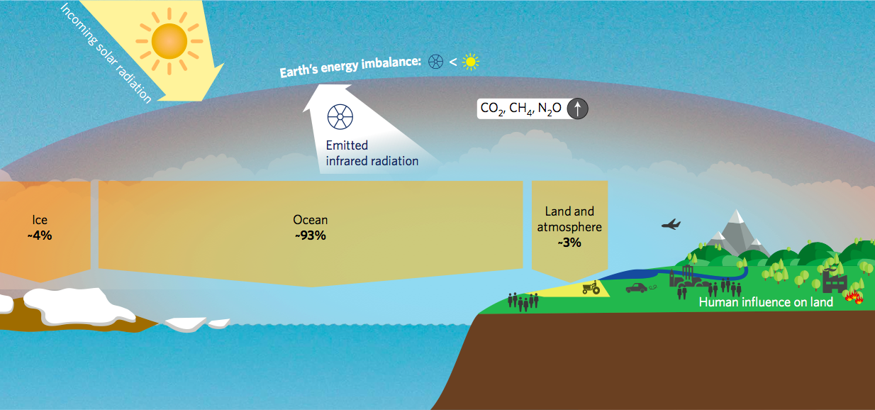
All the energy that enters or leaves the Earth system does so via radiation at the top of the atmosphere. For a stable climate, the sunlight absorbed by the planet must be balanced by thermal infra-red radiation emitted to space. Increased atmospheric greenhouse gas concentrations give rise to an imbalance in Earth’s energy budget by initially reducing the amount of emitted thermal infra-red radiation. The result of this imbalance is an accumulation of excess energy in the Earth system over time. The size of the imbalance, or equivalently, the rate of energy accumulation in the Earth system, is the most fundamental metric determining the rate of climate change.
The vast majority (>90%) of the excess energy is absorbed by the ocean, with much smaller amounts going into heating of the land, atmosphere and ice cover (Figure 1). Therefore, if we want to track the increase in Earth system energy content over time it is essential to have comprehensive measurements of temperature, and the associated heat content, throughout our vast oceans.
The ‘symptoms’ of EEI
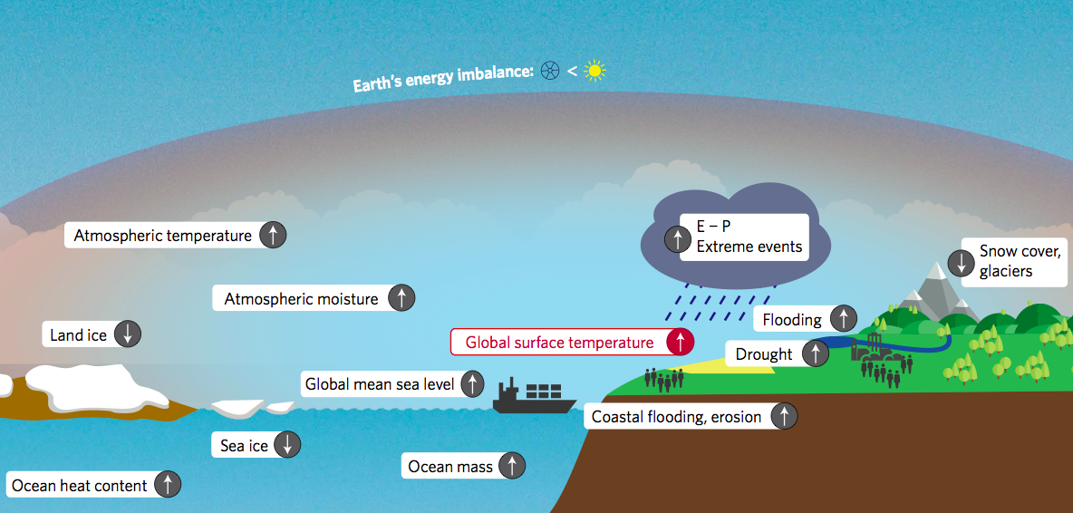
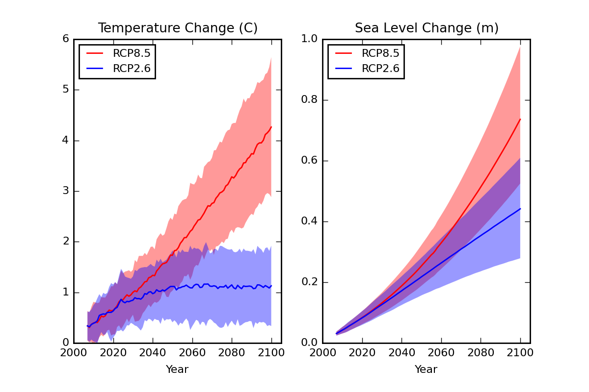
As a result of the energy imbalance, the Earth system adjusts in a number of ways that have a direct impact on both the marine and terrestrial environment. The various elements of global warming that we are familiar with – including global surface temperature rise, reductions in snow and ice cover, and sea level rise – can be thought of as symptoms of EEI (Figure 2). In our thinking and communication around climate change, it is important not to confuse any of these symptoms with the underlying cause.
The global warming ‘hiatus’
A large part of the controversy around the recent slowdown in surface temperature rise, or ‘hiatus’, stems from the fact that many commentators view global surface temperature rise as the primary indicator of global climate change. If surface warming has paused, climate change has paused, right? Wrong. Both observational studies and computer simulations show that there is only a weak relationship between Earth’s energy imbalance and surface temperature change over a decade or so (Figure 3a). This is because natural climate fluctuations can re-arrange ocean heat content, to either offset or add to the long-term rate of global surface temperature rise over a decade or so.
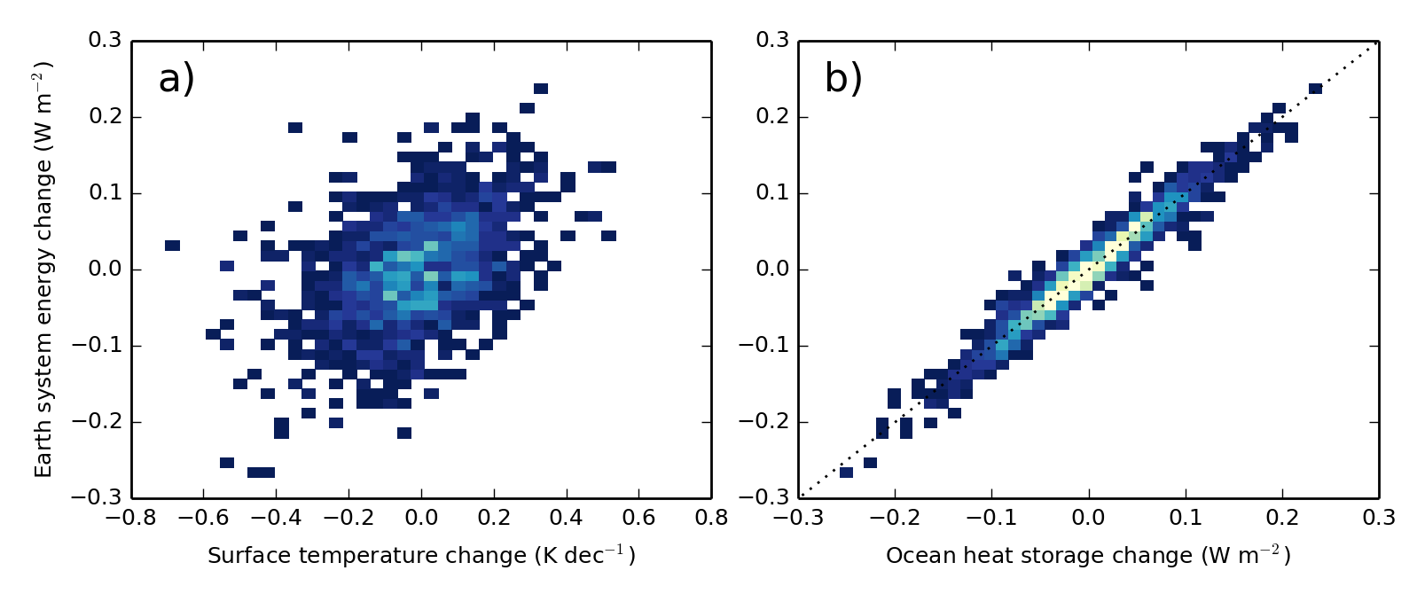
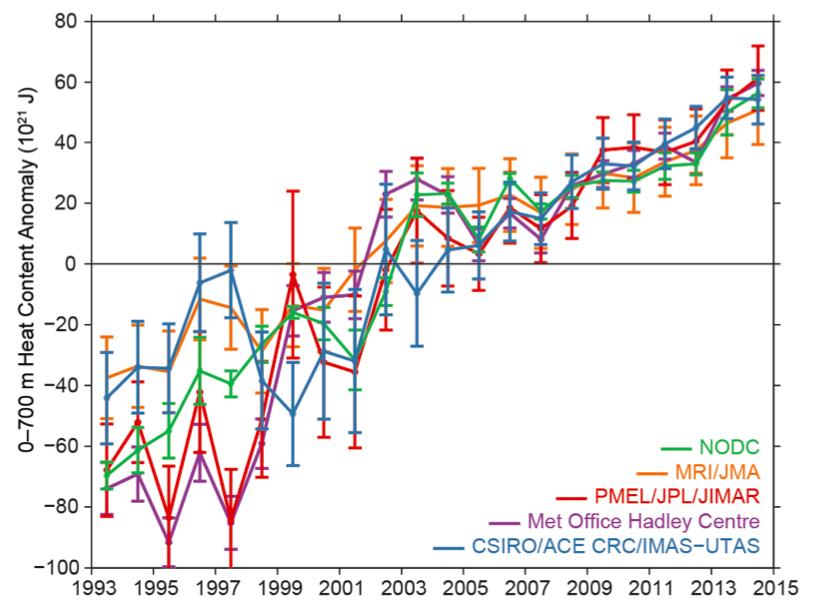
Since the ocean becomes the dominant term in Earth’s energy budget on timescales longer than about 1 year changes in ocean heat content provide a much more reliable indicator of EEI (and therefore climate change) than surface temperature on decadal timescales (Figure 3). Indeed, time series of upper ocean heat content and satellite measurements agree on a fairly steady rate of heat uptake over the past 20 years or so, suggesting that EEI has also been relatively constant during this time (Figure 4). When viewed in terms of EEI, there is little or no evidence for a recent ‘hiatus’ in the rate of global climate change.
How do we measure EEI?
There are three ways in which we can use observations to track EEI and its variations over time. The first is to use satellite measurements of the variations in the radiative energy entering and leaving the Earth system. Second, we can use estimates of heat flows into and out of the ocean surface to infer the EEI because the atmosphere and land have comparably very little heat capacity. The third, and most robust, method is to track the rate of change of Earth system energy storage, which is dominated by ocean heat content for the timescales of interest here.
Each of the methods for estimating EEI has strengths and weaknesses, as discussed by von Schuckmann et al. The most promising strategy for advancing our monitoring capability lies in efforts to combine satellite-based monitoring of variations in EEI with estimates of ocean heat content change. Progress can be achieved through a multidisciplinary community effort to improve both Earth observations and devise optimal methods for combining the information on EEI that they provide.
New observations
An exciting advance under development is the extension of the Argo array of robotic profiling floats to sample the full ocean depth. Argo has revolutionised our ability to monitor changes in ocean heat and freshwater content, since its inception in the early 2000s. However, current generation floats can only sample the upper 2km – roughly 50% of the open ocean depth. New, deeper float technologies are currently in the testing phase and research is being carried out into what this deep array might look like.
Continued monitoring of Earth’s energy balance is paramount for understanding the evolution of climate change and has multi-century implications. Earth will maintain an energy imbalance long after greenhouse gas emissions have been reduced and surface temperature rise has stabilised. One of the important climatic consequences is that global sea level will continue to rise for many centuries after surface temperature rise has ceased, due to the continuing increase in ocean heat content and long term melting of giant ice sheets (Figure 5).
Global surface temperature rise and other key symptoms of EEI are essential foci of climate change science and assessing potential impacts of global warming. However, Earth’s energy imbalance is what ultimately sets the pace of global warming and it should be central to our thinking and communication on climate change.
The authors would like to thank Richard Allan and Jonathan Gregory for helpful suggestions to improve a previous version of this post.
Oh, I thought every scientist already thought GW this way. The trouble has been the exact measurement of EEI. I’d imagine this could be solved if there was a broad spectrum ir sensor at an angle pointed towards the curve of the earth in orbit. This would likely have to be measuring quite a narrow area at a time. I’m not too sure how this can technically be done. Summing up daytime obs and nighttime obs should provide some otherwise hard to obtain data.
Good point. Satellites already measure to good accuracy changes in EEI (to less than a few tenths of a Watt per square metre globally) but to get a reasonable absolute measure of EEI the ocean heating from Argo floats down to 2km and other deeper observations of temperature change are required as discussed in the article. However, more accurate satellite estimates using better calibration and potentially a fleet of tiny satellites are in the planning stage.
Some sort of interpolation of the rss or uah high atmosphere channels might provide some data for this. But probably it’s not accurate enough, as the change in imbalance is so small compared to the overall wattage bouncing around there…
“More than 90% of this imbalance goes into heating the ocean, with much smaller amounts going into melting of ice and heating of the land and atmosphere.
How valid is this statement?
I understand that the capacity of the oceans is much larger than that of other reservoirs, but capacity is not the same as actual transfer.
The largest amounts of mass transfer appear to be cold water creation around Antarctica. What are estimates for diffusive transfer at lower latitudes based on?
It would seem even diffusive transfer must fight buoyancy to transfer heat downward.
I do understand that OHC estimates indicate storage, but I’m also troubled that they don’t currently include measurements for the sea ice covered regions which ( through leads and polynyas ) create the greatest mass exchange.
Thanks for the comment.
I think we can be pretty confident about the ball-park figures for where the energy goes. This is discussed in IPCC AR5 WG1 Chapter 3 on ocean observations, where they present observation-based estimates of the various energy storage terms.
One of the ways we can have more confidence that we’re getting the right answer is through joint analysis of the energy AND sea level budgets – as done by Church et al [2011].
Regarding Antarctic Bottom Water formation, the estimates we have of changes are also based on inventory changes over the global ocean (measuring fluxes directly is very difficult). These are based on full-depth hydrographic sections, which are very sparse in space and time – so the uncertainties are quite big. However, the deeper parts of the ocean (> 2000m) are estimated to make a relatively small, but important contribution to the global energy and sea level budgets – see Purkey and Johnson [2010], for example.
I agree with your comments on ice-covered regions – these are areas we would like to better observe. This may ultimately be addressed through a combination of marine mammal observations and under-ice observations from Argo floats and other platforms. The marginal seas are also poorly observed, in terms of doing a heat inventory.
It would be great to see more work investigating the relative importance of these different regions (ice-covered, deep ocean, marginal seas) for different timescales.
Hi Matt,
Why does your plot of ARGO era 0-700m for 2003-2009 look so different to the plot produced from the data available from the ARGO website prior to 2010?
That data showed a modest decline in 0-700m OHC 2003-2009, but your plot shows a steep rise.
Hi Rog,
I’m not sure which ARGO plot you are referring to?
However, there is a nice article by that has just come out showing a very steady increase in OHC during 2006-2015 – see Wijffels et al [2016] .
I’m referring to your fig 4 compared to data available from ARGO pre 2010. Compare with the plots in this post which used that previously available data.
https://tallbloke.wordpress.com/2010/12/20/working-out-where-the-energy-goes-part-2-peter-berenyi/
Berenyi makes a strong argument here in my opinion. There is a mismatch in the splicing of ARGO data to XBT data in 2003, which inflates OHC. This is demonstrated by the correlation with CERES FLASHFlux net TOA radiation imbalance of ARGO.
Do have a read of that post, it is cogently argued.
Hi Rog,
The CERES Flashflux is a near real time product which is not homogeneous in time and the best CERES data shows fairly constant heating rate with time:
http://www.met.reading.ac.uk/~sgs02rpa/PAPERS/Loeb12NG.pdf
I’m not so sure that’s true.
If it is, there’s no surplus energy left to go into the oceans because the mean net radiance for the period of record of EBAF CERES is near zero.
The measurement uncertainty from satellites is probably a few W/m^2, not tenths of W/m^2, if for no other reason than the anisotropic shortwave variations.
But I suspect the OHC measurements are similarly uncertain because we’re not measuring the areas of the greatest mass exchange ( the polar regions ) very well.
Hello, our collaboration with NASA Langley (who produce the CERES data) show that the combined CERES/Argo record gives a best estimate EEI of about 0.5-0.6 Watts per square metre although with considerable uncertainty relating to the Argo data we used:
http://www.nature.com/ngeo/journal/v5/n2/abs/ngeo1375.html
http://onlinelibrary.wiley.com/doi/10.1002/2014GL060962/full
You’re right that satellite data on their own cannot measure the imbalance to much better than a few Watts per square metre. However, their stability of measurement is much better and can observe changes in the net imbalance to less than a few Watts per square metre so we can track how accurately the imbalance changes over time using CERES and the growing Argo record provides the absolute value of the imbalance.
Thanks for your replies Richard. From your second link:
“Curiously, the ocean heating rates during the early 2000s measured by ocean reanalyses and ocean heat content data sets reach values greater than 1 Wm−2 [Trenberth et al., 2014], which is similar in magnitude but opposite in sign to the changes following large volcanic eruptions or large El Niño events. Trenberth et al. [2014] show that N is reduced following El Niño events, while N typically increases following La Niña conditions, which were not present during the 2001–2005 period (Figure S7). Such large values of N in the early 2000s are also not present in the CERES record [Loeb et al., 2012], and this discrepancy merits further investigation.”
Is this not suggestive of a problem with the splicing of XBT to ARGO datasets around 2003? The post on my site I linked earlier found the same problem using the CERES data in concert with the OHC time series.
Southern hemisphere SST shows a decline 2003-2009 which doesn’t appear in ARGO data any more.
plot
Hello again, you’re right there is certainly something funny in the ocean data around 2003 but there is also a drop in the XBT quality:
http://onlinelibrary.wiley.com/doi/10.1002/2014GL062669/full
The combined satellite/Argo record suggests a slight drop in EEI from the late 1990s-early 2000 but otherwise quite stable at around 0.6 Watts per square metre of heating with variations due to ENSO.
For the period 2001-2010, perhaps.
But for the period of record ( March 2000 through March 2015, still waiting for the latest ) – close to zero mean of net radiance.
Now, zero is not inconsistent with 0.5 to 0.6 W/m^2 because of the uncertainty.
But, it’s also not inconsistent with zero.
Hello again, where do you get your CERES time series data? The CERES team who produce the data get about 0.6 Watts per square metre on average (see Table 2):
http://link.springer.com/article/10.1007/s00382-015-2766-z/fulltext.html
You can get the CERES data from their website (they use geodetic weighting to accurately calculate the global averages) but you can also get pre-computed global means which you must annual average to get a meaningful EEI:
https://ceres-tool.larc.nasa.gov/ord-tool/jsp/EBAFSelection.jsp
Hi Richard,
The data used was digitised by Berenyi from online NOAA plots. The file is here
http://ber.parawag.net/images/OHC_and_TOA_net_imbalance.csv
Cheers
Matt Palmer and Doug McNeall – I was just alerted to your weblog.
I am really glad you are doing this. This research is, in my view, a game-changer.
As both of you know (but your readers may not), I recommended this replacement of the global average surface temperature trend with the assessment of ocean heat content changes in my papers:
Pielke Sr., R.A., 2003: Heat storage within the Earth system. Bull. Amer. Meteor. Soc., 84, 331-335. http://pielkeclimatesci.wordpress.com/files/2009/10/r-247.pdf
Pielke Sr., R.A., 2008: A broader view of the role of humans in the climate system. Physics Today, 61, Vol. 11, 54-55. http://pielkeclimatesci.wordpress.com/files/2009/10/r-334.pdf
The introduction to your post
“Surface temperature rise is often thought of as synonymous with climate change. However a recently published paper in Nature Climate Change argues that Earth’s energy imbalance (EEI) is what ultimately sets the pace of climate change and that substantive progress can be made by monitoring this key climate variable.”
is an excellent framework to finally move beyond surface temperature. While I have concluded “climate change” is much more than just changes in the energy imbalance, in terms of global warming this is the way to move forward. Figure 3 that you present in the post is a succinct, extremely important result that should be widely cited.
I look forward to following your research. Among the questions are
1. Do the climate models replicates the observed hemispheric asymmetry in ocean heat accumulation?
2. How did the heat start being transferred to depth without being sampled in the upper ocean? Why did this deeper ocean accumulation start later in the record?
3. What is the heat accumulation within the layer between the thermocline and the surface and how does this compare with the model predicted accumulation?
4. Once heat is at depth, how would it reemerge into the upper ocean on multi-decadal time periods?
5. How was the heat accumulation in non-sampled regions estimated?
6. In http://pielkeclimatesci.files.wordpress.com/2009/09/1116592hansen.pdf by Jim Hansen, he wrote
“The decadal mean planetary energy imbalance, 0.75 W/m2 , includes heat
storage in the deeper ocean and energy used to melt ice and warm the air and land. 0.85 W/m2 is the imbalance at the end of the decade.” [meaning the 1990s].
Does this indicate that the GISS model is predicting higher global warming than the observations? Are their updated GISS results that can be checked?
Best Regards
Roger Sr.
Crickets
Thanks for the comments and questions Roger.
I’ll try to provide some input on some those questions..
Hemispheric asymmetry is indeed seen in climate projections of ocean heat uptake – see for example the work of Kuhlbrodt and Gregory [2013] – we know that the Southern Ocean is particularly important for heat uptake.
We need to do more work to understand the observed ocean heat content changes, and this is something that several groups are currently working on. The turbulent nature of the ocean and small-scale “noise” from the mesoscale eddy field make this a challenging problem from a sampling point-of-view. As shown in the Wijffels et al paper linked above, ENSO activity introduces systematic variations in OHC over the upper few hundred meters that somewhat obscures the longer-term variations.
In any case, it is not obvious to me that any warming signal would translate smoothly into the ocean interior – some of the key processes of ocean heat content change, i.e. those associated with water-mass-formation – are seasonal and often episodic (e.g. convection at high latitudes).
The recent study by Gleckler et al [2016] presents a comparison between CMIP5 models and historical observations of ocean heat content change. The multi-model-mean shows remarkable agreement with the available observations across 3 different depth layers, but there is considerable uncertainty – due to both the inter-model differences, and limited sampling in the observations.
Hope that helps..
A lay comment: if about ~93% of the energy imbalance is going into the sea, why not estimate it via thermal expansion of the sea? climate.nasa.gov/vital-signs/sea-level/ says 3.4mm per year. A metre cubed of seawater expands 0.25mm vertically per K, that is per 4.2 MJ. That means 57 MJ year^-1 m^-2, or and energy imbalance 1.8 Wm^-2. I know melting sea ice will reduce the rise, and land melt increases it (land melt requires only 2% of the energy to produce the same rise?), but doesn’t that imply we should improve accuracy of glacier melt etc? Would be great to get more measurements all round.
Hi,
Could someone please confirm for me that the rising ocean temperatures are buffered by the cooling effect of the polar ice sheets? If so, is this heat transfer equilibrium taken into account when making extrapolations? My fear is that the ice heat buffer is being used up and once gone, it would only be a matter of a year or so before we would see meteoric ocean temperature rises. Think ice cubes put into hot water with a heat source. Everyone talks about sea level rise and thus implies to the public that this is the gravest effect of icemelt, but the effects of ocean temperature rise would be catastrophic for ocean food sources and weather systems due to vastly increased water levels in the atmosphere. Am I wrong to be so concerned?
Interesting question, Ashley. I don’t know the answer (non-expert) but the same thing occurred to me, specifically about sea ice, which seems to be in contact with water more, so could be a more effective ‘buffer’. Greenland glaciers and sea ice seem to be each losing hundreds of gigatonnes per year.
If there is an increase in snowing on a land sheet, it would presumably warm surrounding seas, but while it is melting, it is cooling. I recall a couple of papers suggesting sea ice melt is happening faster than models predict from the rise in temperature itself. What’s that, a few 10^19 J/year, so only a hundredth as much heat going into the cryosphere as the oceans (probably my calculations are wrong, as I’ve seen it as a few percent) . Sea temperatures are not rising that fast below the surface though, and it seems a complete loss of the cryosphere wouldn’t add to the rate more than a few percent.
What I would worry about as regards ice though is the change in albedo. It’s not a greenhouse effect, but means Earth has to radiate significantly faster.