Much evidence has accumulated that temperature extremes and variability are changing. Accurately diagnosing such changes is of vital societal interest, not least because human induced climate change is often expected to materialise primarily through changes in the extreme tails.
Quantifying these features of climate time series statistically in climate models and observations is not straightforward. To a large extent, that is because extreme events are rare by definition, a fact that seems hardly surprising. This fact implies, however, that conventional methods quickly break down when it comes to the tails. This blog post serves s a cautionary note, in which we discuss how apparently very simple methods can result in severely biased estimates, and how this can be avoided1,2.
Guest post by Sebastian Sippel, MPIB, based on Sippel et al. (2015)
Many studies that take on global or continental-scale perspectives circumvent this “small-sample” issue by counting extremes across space, which results in a metric such as the “global land area affected by temperature extremes” (or similar ones). However, an ‘objective comparison’ across space requires a transformation based on the local statistical properties of the time series, because locations differ in their climatic means and variability. A conventional approach that has been termed ‘reference period normalization’ is to subtract the long-term mean and divide by the standard deviation of a time series estimated in a ‘climatic reference period’ (assuming Gaussianity), yielding standardized (‘comparable’), bell-shaped estimates for climatic variables across space.
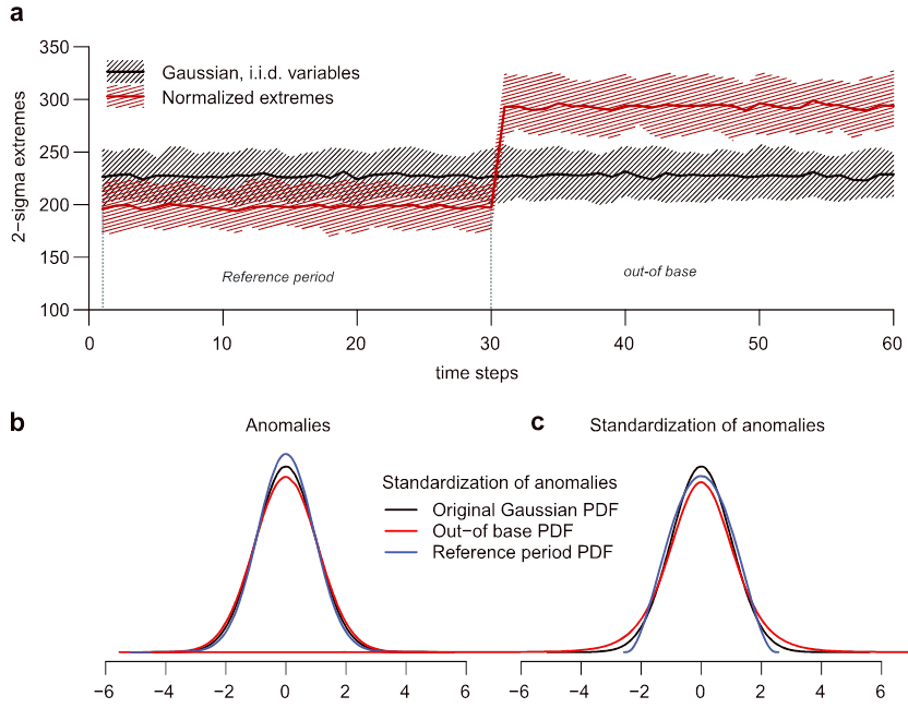
However, a simple experiment with artificial and stationary Gaussian data shows that the approach breaks down when it comes to the extremes (Fig. 1a, extremes defined as exceeding a certain level of variability, i.e. ‘sigma-extremes’): The number of extreme events increases drastically from the period that was used as reference period to the non-reference (‘independent’) period. These artefacts are more severe for short reference periods and more extreme extremes (e.g. an artificial increase in observed extremes by 48.2% for 2-sigma events in a n=30 year reference period), but more importantly the issue holds generically.
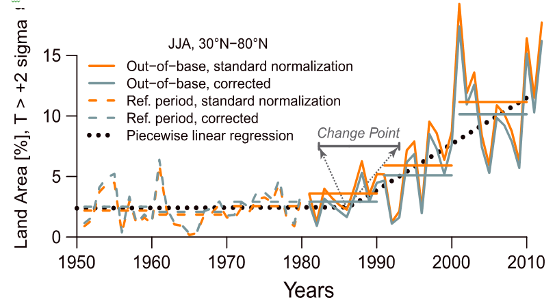
The reasons for these apparent methodological problems are statistically surprisingly simple: the estimators of mean and standard deviation have been calculated from values taken from the reference period – therefore the normalization transformation is conducted using dependent estimators in the reference period, and independent estimators outside. From a statistical point of view, it is well known that such operation yields different ‘normalized’ distributions (Fig. 1b and 1c) – in this case, it would result in a so-called beta- and t-distribution within and outside the reference period, respectively. Importantly, these distributions differ considerably in the shape of their tails – leading to the observed inconsistencies in the number of extremes across time and space. These findings have led to a downward correction of previous studies1 quantifying the number of summer temperature extremes across the Northern hemisphere2 (Fig. 2).
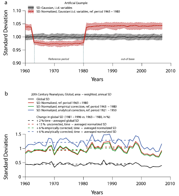
Furthermore, this statistical issue extends to estimates of the normalized climatic variability, because different statistical distributions entail differences in their variances (Fig. 3a). Therefore, accounting and correcting for the normalization issue shows that in contrast to previous reports3, both global and normalized temperature variability has not increased at the global scale (Fig. 3b).
To summarize, caution is required when estimating properties of climatic time series in one ‘reference’ part of the series, and subsequent application and analyses on the entire series. This finding is not new4 – but given abundant recent interest in climatic extremes, data analytic tools and indices require careful reconsideration in light of this issue.
References:
1. Hansen, J., M. Sato, and R. Ruedy (2012), Perception of climate change, Proc. Natl. Acad. Sci. U.S.A., 109, E2415.
2. Sippel, S., J. Zscheischler,
M. Heimann, F. E. L. Otto, J. Peters,
and M. D. Mahecha (2015), Quantifying changes in climate variability and extremes: Pitfalls and their overcoming, Geophys. Res. Lett.,
42.
3. Huntingford, C., P. D. Jones, V. N. Livina, T. M. Lenton, and P. M. Cox (2013), No increase in global temperature variability despite changing regional patterns, Nature, 500, 327.
4. Zhang, X. B., G. Hegerl, F. W. Zwiers, and J. Kenyon (2005), Avoiding inhomogeneity in percentile-based indices of temperature extremes, J. Climate, 18, 1641.
Interesting thought. However, I wonder how often the method that is critiqued is actually used. I will not claim to know the literature on this very well, but I do not think that I have come across an article that first computes anomalies and averages them before they study changes in extremes.
I could imagine people doing this wrong and that warning them is valuable, because the main reason this does not happen much is likely that the most extreme extremes are at the local level and that studying them is hard enough, thus people currently do not often average before studying extremes. (This may change because also extremes at different spatial (and temporal) scales are important.)
The “climate dice” article of James Hansen could have been an exception, but he claims he did not want to draw conclusions about changes in variability. As I wrote at the time:
This weekend I was reading a potential one: the controversial paper by James Hansen et al. (2012) popularly described as “The New Climate Dice“. Its results suggest that variability is increasing. After an op-ed in the Washington Post, this article attracted much attention with multiple reviews on Open Mind (1, 2, 3), Sceptical Science and Real Climate. A Google search finds more than 60 thousand webpages, including rants by the climate ostriches.
While I was reading this paper the Berkeley Earth Surface Temperature group send out a newsletter announcing that they have also written two memos about Hansen et al.: one by Wickenburg and one by Hausfather. At the end of the Hausfather memo there is a personal communication by James Hansen that states that the paper did not intend to study variability. That is a pity, but at least saves me the time trying to understand the last figure.
Hi Victor,
thanks very much for your comment.
Indeed, most studies looking at extremes using e.g. extreme value statistics or similar methods circumvent this issue by studying extremes at any one particular place (and thus are not affected by the issue discussed here).
However, there are also a number of studies that pursue the methodology described above (have a look in the paper that indicates several studies, but there might be more).
Just to clarify, the methodology is not about averaging after computing anomalies, but about counting “z-transformed extremes (e.g. sigma-events)” across space (i.e. not averaging all anomalies/z-scores, but the extreme ones).
Regarding your last point:
It’s still worth to look at the last figure, as it shows that this also cause some issues in calculating “normalised variability” across space. It’s true that the Hansen et al (2012) paper mainly studied extremes. However, a subsequent paper that appeared in Nature a year later (Reference 3 above) studied changes/trends in the absolute and normalised temperature variability, and here the “normalisation issue” is indeed very relevant.
Best wishes
Sebastian
Yes the troubles with the ends of the dataset prevent strict separation of analysis methods. Say you calculated your baseline as being the moving 30-year average, even with a good smoothing in the ends (such as Lowess) then the most recent (and most early) extreme values could be omitted or accentuated very easily. Then your most valid analysis would end 15 years before the dataset. I see no way around this problem with the moving baseline. This makes it hard to say what exact part of warming is made by ENSO and what by AGW, f.e. Fer sure, both have a say in the low troposphere temperature series, but the division between them is the thing. Thus your image with linearized baselines might make sense since I think this might, in the end give a better constant error… anyway waiting 15 years for a theory to be confirmed isn’t unheard in science, so one might as well give it a go…
“…human induced climate change is often expected to materialise primarily through changes in the extreme tails.”
Seems to me that one might expect less temperature variability and reduced extremes with a CO2 enriched atmosphere.
The reason being that a water vapor feedback would increase the latent heat content, meaning that less sensible heat transfer is necessary to resolve spatial energy imbalances.
This certainly holds true for the examples we have: summers have less temperature variability than winters and spatially, the Tropics have less temperature variability than the Temperate and Polar zones.
“Much evidence has accumulated that temperature extremes and variability are changing”
Not necessarily so:
http://www.nature.com/nature/journal/v500/n7462/full/nature12310.html for instance
Would you be able to help dissuade me of an idea. It is on the theme of statistical artefacts but in very broad way. I am not claiming any validity to this idea , I just wondered if someone can show me the flaw, and explain where I am going wrong.. or if even if there is an outside chance I am right?
until amazingly recently sea surface temp was taken by swinging a bucket over the side of a ship. This is the form of record taking from the mid 1800s The type of bucket varied from metal , wood to leather. The depth it was taken from was inconsistence and even what side of the ship and the length of time it was left waiting before some ship hand stuck a thermometer in it would change the reading dramatically.
So obviously this is a terrible method for measuring temperature.
It is still though a record gained from direct recordings. All other temperature records are inferred from proxy sources.
When data is inaccurate it is not disregarded but instead an error bar is applied, these are the red and yellow wiggly lines that track either side of the climate graph.
The greater the chance of inaccuracy the greater the error bar.
If you look at the graph you will see that these error bars are narrow from 1970 but get get dramatically wider before this date.
so the explination for this sudden narrowing of the data bar around 1975 is… the cold war.
The US were obsessed with finding out what thermal nuclear bombs the Russians had, so they deployed a global network of sophisticated weather bouys . These accurately measured the temperature so they could detect changes and infer the nuclear capacity of the Russians.
he significant factor of man made global warming is that it is far more extreme than previous changes in global temperature. The hockey stick graph shows a sudden and unrelenting rise in temperature from the mid 70s on. This an unprecedented change and can only be acounted for by human activity. previous swings in temperature were much much slower.
But
pre 1970 temperature estimations had a large amount of inaccuracy. The correct thing to do with this inaccuracy is to homogenise the data. Scientists correctly take all the extremes and average it out, this gives a nice smooth flowing , gently undulating climate graph that reflects the trends in temperature over time.
But we are using the sudden dramatic change in temperature as our main signifier.
Post 70s data is extremely accurate, this is unintended byproduct of the cold war paranoia.
This information does not need to be homogenised (averaged) to such an extent. It will still contain an error bar but only that which is reflective of the proportion of inaccuracy contained in the method.. so not much.
So what I believe is happening is the switch between data collection is creating a statistical artefact. The truth about climate is not the one being presented. Earths temperature did not undulate gradually for thousands of years and then suddenly shoot up in the 70s. Instead this the climate has always been in this state of extreme flux. Massive peeks and troughs throughout our history, exactly as we are currently experiencing.
Interestingly many different sources of proxy evidence, tree rings , pupa emergance, coral records seem to diverge from the official chart from the 1970s on. in each case the biological process is forced to change to fit the climate data. Its as if the chart is sovereign and all other methods must change. Tree growth was seen as a reliable proxy untill it divergerd at this date.then a new mechanism had to be applied, water was considered the main factor. Butterfly emergence had to be changed from this date, suddenly a time cut off was applied.
Biological evidence is thrown out or modified when it doesn’t apply and used when it supports.