The latest global climate models (GCMs) have performed pre-industrial control simulations as part of the CMIP5 coordinated experiments. In these simulations there are no changes to radiative forcings, which are kept fixed at year 1850 values – all the variability is therefore generated internally to the climate system. How different can this variability be?
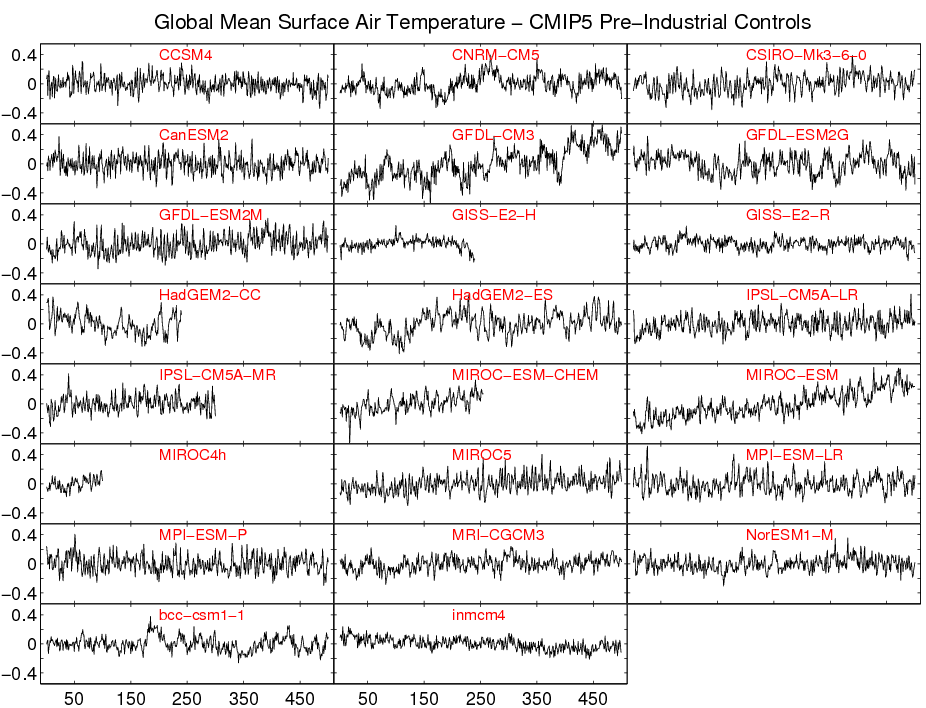
The first post on this blog compared the pre-industrial control simulations from the previous CMIP3 GCMs. The figure below updates that comparison to CMIP5 – the same scale is used for each simulation.
It is instantly clear that there are large differences in simulated internal variability, just like in CMIP3. Several models have very little variability (e.g. GISS, inmcm4), others have significant decadal variability (e.g. GFDL CM3, CMCC-CM), and some have ‘drifts’ because they have yet to reach equilibrium (e.g. GFDL CM3). By eye, the amplitude of inter-annual variability in the observations sits between the extremes from the simulations, perhaps towards the lower end, but separating out the variability from the trend is non-trivial.
What should we make of this? Much of the difference in simulated inter-annual variability is likely due to different ENSO variability characteristics, but the decadal variability is likely to reside elsewhere, perhaps in the Atlantic or extra-tropical Pacific Oceans? Maybe that will be next to look at.
The enormous differences in time series alone are very beautiful.
Some time series look intermittent, where the beginning shows little decadal variability and after some time it starts. Could be that not only the mean, but also the variability needs a spin up?
It would be great to see some structure functions of these graphs; an analysis method often used in turbulence research, another complex system. The second order structure functions are equivalent to the power spectrum, the higher orders focus more on the structure of the larger jumps in the series. If the structure functions are reasonably well approximated by power laws, it may be possible to classify the models based on their exponents. AR coefficient are mainly determined by the shortest time scales, the interannual variability, with power spectra and structure functions you would see the long term (including decadal) variability clearer.
It would be interesting to have a look whether the models with a deep ocean and a high atmospheric top show more decadal variability. For the COSMO model, the spatial structure differs a lot between the two numerical solvers (Runge-Kutta and Leap-Frog). I would not expect that this percolates to the temporal structure of the global means, but still it may be interesting to see if the numerical solver can explain some of the differences in structure.
If I perform the trivial action of rotating my head somewhat when looking at the observations to remove the trend then by eye I’m left with variability the looks more like GFDL than GISS. Especially if some part of the last 30 years of obs is akin to one those decadal long excursions seen in GFDL variability rather than all being trend.
Is this a revelation of the ability of the climate models to reveal the ‘fingerprint’ of anthropogenic global warming, or is it a revelation of the consistent lack of skill of climate models to simulate natural external and internal decadal forcings?
We have a clue as to the answer when we take the alternative view of comparing climate models with observations of global temperature for the last 15 years or so – virtually all of them consistently fail to predict the observed slowdown/pause in global temperatures, meaning it is very likely that they all consistently have failed to model some aspect of natural climate variability.
Of course, some aspects of natural variability can never be modeled, like volcanic eruptions and changes in solar irradiance. Both are thought to have contributed to the slowdown of the last 15 or so years, especially the former.
Hi David,
Those processes can be, and are, modelled. But they can not always be predicted ahead of time. But, we can provide ranges for future given plausible eruptions and solar changes.
Cheers,
Ed.