As the attention received by the ‘global warming hiatus’ demonstrates, global mean surface temperature (T) variability on decadal timescales is of great interest to both the general public and to scientists. Here, I will discuss a recently published paper (Brown et al., 2014) that attempts to contribute to this scientific discussion by investigating the impact of unforced (internal) changes in the earth’s top-of-atmosphere (TOA) energy budget on decadal T variability.
Guest post by Patrick Brown (Duke University)
Figure 1 illustrates a very simple (but hopefully still useful) way to think about T change. In this model, T changes as a result of an energy imbalance (Qnet) on the system composed of the land, atmosphere and ocean’s mixed layer. Specifically, T change results from an energy imbalance at the TOA (QTOA, which is the difference between Reflected Shortwave Radiation (RSW) plus Outgoing Longwave Radiation (OLR) and Incoming Shortwave Radiation (ISW)) and/or at the bottom of the ocean’s mixed layer (QBML, positive up). Obviously there has been a great deal of research on T change associated with externally forced changes in QTOA (Category A in Figure 1; Myhre et al., 2013). Also, there has been quite a bit of research recently on decadal T change resulting from unforced variability in the exchange of heat between the ocean’s mixed layer and the ocean below the mixed layer (Category C in Figure 1; England et al., 2014; Balmaseda et al., 2013; Meehl et al., 2013; Trenberth & Fasullo, 2013). In our reading of the literature, however, less attention has been given to decadal T change associated with unforced changes in the TOA energy budget (Category B in Figure 1). This is the topic of Brown et al. (2014).
I should note here that Spencer and Braswell (2008) stressed the importance of non-feedback TOA radiation variability on T change but that this is a slightly different focus than our study because we were not concerned with distinguishing between feedback-related and non-feedback related TOA imbalances. The study that is most closely related to our own is probably Palmer & McNeall (2014) and many of our results are complementary to theirs.
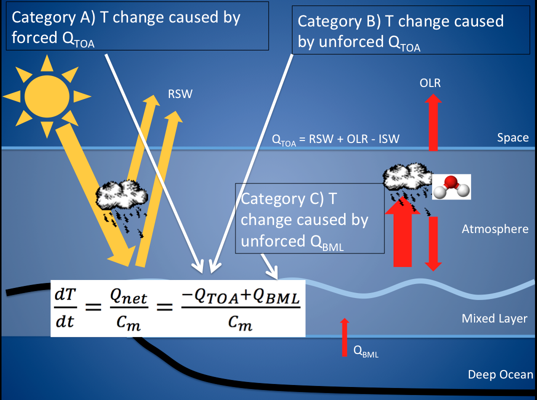
We investigated unforced control runs from the CMIP5 archive and looked at what the TOA energy budget was doing during decades when the models spontaneously simulated large changes in T (since these were unforced runs, there was no Category A variability, by definition). We found that unforced, decadal changes in T tend to be enhanced by TOA energy imbalances. In other words, during large-magnitude warming decades, the net flux at the TOA tended to be into the climate system and during large-magnitude cooling decades the net flux at the TOA tended to be out of the climate system. How much did the TOA energy imbalances affect temperature? We used published effective heat capacities of many CMIP5 models (Cm in Figure 1) to estimate that the TOA flux during these decades was responsible for approximately half of the change in T on average (the other half would be due to QBML).
It may seem counter-intuitive that the net flux at the TOA would enhance (rather than reduce) T change because the Stefan–Boltzmann law might lead us to expect that as T decreases (increases), the amount of outgoing longwave radiation emitted to space should decrease (increase) exponentially.
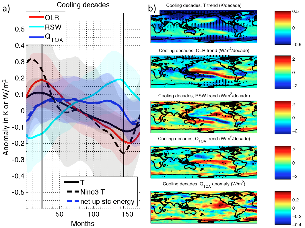
Figure 2 shows the temporal (Figure 2a) and spatial (Figure 2b) variability of temperature and energy flux variables over large-magnitude cooling decades. It can be seen that outgoing longwave radiation does in fact decrease during cooling decades but that the net TOA energy flux remains positive (out of the climate system) for most of the decade because reflected shortwave radiation tends to increase by roughly the same amount as outgoing longwave radiation decreases (Figure 2a). In other words, it appears that changes in the climate system’s albedo are able to temporarily counteract the changes in outgoing longwave radiation and thus sustain the net TOA imbalance for a longer period of time than might be expected otherwise. We find that these changes in albedo appear to be associated with changes in the state of the Interdecadal Pacific Oscillation (at least in the multi-model mean pattern). In particular, reflected shortwave radiation over the equatorial and eastern Pacific tends to increase as surface temperatures over that region decrease (Figure 2b).
These model-based findings appear to contradict observations over the past 10-15 years. In particular, it has been suggested that we are currently in an unforced cooling situation analogous to that illustrated in Figure 2 (e.g., England et al., 2014; Trenberth and Fasullo, 2013). These findings suggest that we should expect this unforced cooling to be enhanced by the net energy imbalance at the TOA (i.e., there should have been a decrease in the rate of climate system heat uptake over this period). However, our best inventories of total climate system heat content have indicated that just the opposite has occurred (as T has been in an unforced cooling state, the rate of climate system heat uptake as increased; Trenberth and Fasullo, 2013; Balmaseda et al., 2013). This is not what the CMIP5 models typically do, but it does happen (~13% of the cooling decades investigated were associated with net positive climate system heat uptake). In these rare decades, changes in QBML flux are large enough to overcome the gain in climate system energy and cause T cooling. This does seem consistent with the recent finding that an increase in Pacific trade wind strength has increased the rate of heat storage below the mixed layer (QBML) to unprecedented levels (England et al., 2014).
This study may raise more questions than it immediately answers and we hope to learn a great deal more as we dig into the results further.
Brown, P., Li, W., Li, L., & Ming, Y. (2014). Top-of-atmosphere radiative contribution to unforced decadal global temperature variability in climate models Geophysical Research Letters DOI: 10.1002/2014GL060625
Thanks Ed and Patrick for this posting! Saves some time as it nicely sums up the gist of the paper. You may allow me one brief comment. Given that the planet didn’t actually cool (in fact, the only interval with stagnation is 2002-2013, but no cooling), the observed increase in the net energy imbalance at TOA might be less contradicting than it appears. I might be wrong, but at least that was my immediate thought upon reading your concluding paragraph. In essence, unforced cooling and forced warming just about counterbalanced each other for the last 10-12 years, such that the forced component can be made responsible for the observed TOA imbalance. Does that make sense?
Hi K.a.r.S.t.e.N
Thanks for the comment.
I should clarify that we do not necessarily expect the climate system to be loosing energy over the past 10-12 years just because we have been in an unforced cooling episode. As you say, the forced imbalance (into the system) could overcome an unforced imbalance (out of the system) and cause the observed imbalance to be into the system. What is contradictory is that we would expect the observed imbalance (into the system) to decrease when we are in an unforced cooling episode and it appears as though it has only increased. This, of course, assumes that the background forced imbalance has been relatively constant which may not be the case.
I should further clarify that when I say “unforced cooling” I mean cooling relative to the forced change, not absolute cooling. So an unforced cooling event would be a time when we are warming at a reduced rate compared to the forced change.
“We used published effective heat capacities of many CMIP5 models (Cm in Figure 1) to estimate that the TOA flux during these decades was responsible for approximately half of the change in T on average (the other half would be due to QBML).”
Is there any reason the partition should be 50-50, or did it just happen that way?
Hi Robert,
In the way that we conceptualized the problem (equation in figure 1 above), all the energy that goes into changing T must come from either the top of the atmosphere or from the bottom of the mixed layer so if 50% came from the top of the atmosphere than the other 50% “must” have come from the bottom of the mixed layer. This is just a 1st order estimation of the flux contributions from each source and future work will need to investigate the magnitude of smaller terms that could effect this calculation (e.g., how much energy goes into melting ice during warming decades).
Also, we calculate that the flux from the top of the atmosphere is responsible for ~50% of the temperature change on average but there is huge variation from decade to decade (Figure 2 in the actual paper).