There has been much discussion recently on whether GCMs participating in intercomparisons, such as CMIP3 and CMIP5, are ‘independent’. But if they are not, how does this make a difference to the uncertainty in our projections for future climate?
The usual measure of spread of GCM projections, as estimated by the variance, assumes that the GCMs are independent. Jewson & Hawkins (2009) demonstrated that, assuming the same ‘correlation’ (r) between all GCMs, the variance should be inflated by a factor of 1/(1-r) to account for the non-independence.
We do not yet have an estimate of the non-independence for future projections (suggestions welcome!) – as it is not simply the correlation between the temperature timeseries. However, a recent estimate of the non-independence of GCMs using the spatial patterns of biases compared to recent observations has suggested an r of around 0.5. However, the IPCC AR4 ‘likely’ ranges for each scenario were given as the mean-40% to mean+60% – which roughly equates to a r of around 0.75.
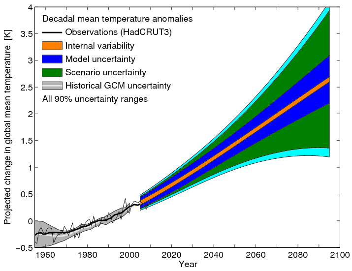
An estimate of the additional model response uncertainty produced by the non-indepedence, assuming r = 0.5, is shown by the cyan region in Fig. 1 below, updating the figure from Hawkins & Sutton (2011). So… uncertainty in uncertainty.

Hi Ed,
Interesting blog!
I’m not sure how to interpret your usage of correlation, however (assuming your derivation of an inflation factor is correct) the pairwise correlation of errors, as Knutti et al calculated, certainly cannot be the same thing. See Annan and Hargreaves GRL 2010 and JClim 2011 – especially the Appendix of the latter, in which we showed that a perfect forecast (which needs neither inflation nor shrinkage) would have typical error correlation of 0.5. And FWIW, Yokohata et al JClim in press confirms our speculation in the JCLim paper about the HadSM3 ensemble (and in fact several other single model ensembles) seeming relatively narrow according to the simple rank histogram analysis.
Thanks James!
I’m not entirely sure how to interpret the correlation either! My feeling was that it may be possible to relate the effective number of models as derived by Knutti et al or Pennell & Reichler into some inflation factor. However, you are suggesting that looking at the historical biases says little about the future performance of the ensemble? Is it then perhaps possible to determine the effective number of models solely from the future projections instead I wonder….
Ed.
I’m just saying that this exploration of biases doesn’t actually mean what many people take it to mean. Do the same analysis on a well-calibrated NWP forecast (or any artificial perfect system) and you’ll see that it has an error correlation of 0.5!
I’m also surprised how many people seem to take that rather silly Pennell and Reichler paper seriously…