Uncertainty in climate projections arises from several different sources. For example, the future emissions scenario is not known, so the usual approach is to run several to compare plausible futures. In addition, each climate model produces a different change in climate. However, on regional spatial scales and for the next couple of decades, it is the internal variability of climate which dominates. These natural climate fluctuations provide an irreducible limit on the precision with which we can make predictions on such spatial and temporal scales – but how large is this limit?
Several recent papers have considered this issue, and an example has been previously discussed here. One approach is to run multiple simulations of the future using the same model and scenario, but with different initial states. In the simplest case, the initial state only differs by a tiny perturbation which grows with the chaotic evolution of the atmosphere (i.e. the butterfly effect). The differences in simulated future climate can be surprisingly large – and this is the irreducible limit as we cannot predict the chaotic atmospheric fluctuations. On global scales, this limit is small, but it can be a large effect on regional scales, and for more variable aspects of the climate, such as precipitation.
One open question from such studies is the importance of the particular ocean state chosen for such an experiment. It is likely that starting the simulations from a range of ocean states would produce a wider spread in projections. It is also possible that using a single ocean state might bias the answer because of the memory in the initial conditions – the future spread (and even the mean) might depend on the initial conditions.
To address these issues, we have adopted a more idealised approach. We are using the fast FAMOUS climate model, which has a coarse spatial resolution, to run larger ensembles than have previously been possible. We are also using an idealised 1%/year increase in CO2 as our scenario. This limits the real world applicability of the results, but is designed to highlight the potential implications.
We first selected 30 different ocean states from a long ‘control’ simulation and ran 140 years into the future from each state using the same 1%/year scenario – this is termed the MACRO ensemble. We next selected 3 of these ocean states and ran 50 (and in one case 100) members, each with just a different tiny perturbation to SSTs in a single grid point, all with the same scenario. These were the MICRO ensembles.
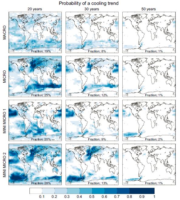
As a first comparison, Figure 1 shows the probability of the first N years of the simulation to show a cooling – i.e. a negative linear trend. The MACRO ensemble, which samples a range of different ocean initial condition, shows a relatively even probability for many locations – for example, around 20% in the extra-tropics for the first 20 years. Interestingly, the different MICRO ensembles show larger probabilities, but only in certain locations, and these locations differ. This highlights that the particular ocean state chosen in each case provides some memory to the subsequent evolution. It also emphasises that if we can use knowledge of the current ocean state we may be able to constrain our projections, which normally adopt a MACRO approach. For longer trends, the probability decreases as expected and the patterns become more similar as the ocean memory is lost.
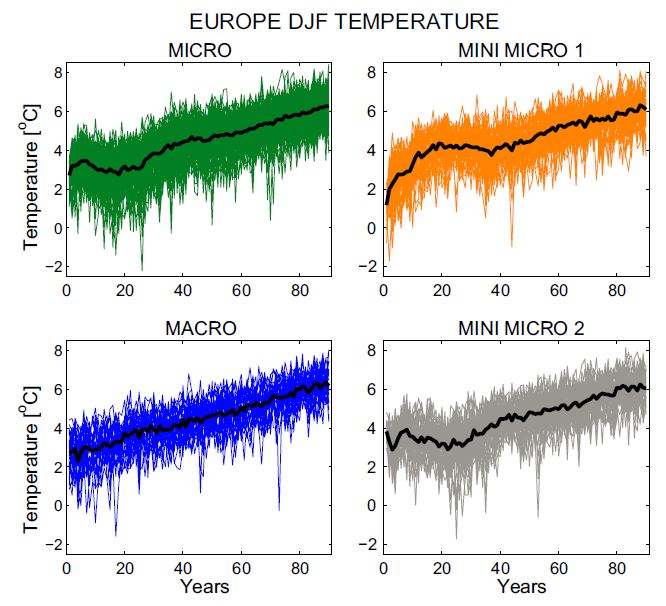
As a specific example, if you live in Europe, you either have a 0% or 50% chance of a cooling over the next 20 years, depending on the ocean state. Figure 2 shows all the timeseries for winter (DJF) over Europe in the various ensembles. The differences are clear by eye – for particular different ocean states there is a high chance of a warming or a cooling over the first couple of decades! This memory is encouraging for the predictability of climate on these timescales. For the MACRO ensemble – which is more akin to the usual climate projections – the warming is more even.
To further illustrate the differences between the ensembles, Figure 3 shows the histograms of trends over the first 20 years of the simulations for European winter temperatures. The MACRO ensemble shows the widest spread as it uses a range of ocean initial conditions. The individual MICRO ensembles show different spreads, suggesting that the uncertainty in future projections is dependent on the initial state. And, in the case of the MINI MICRO ensembles, they hardly overlap!

Lessons learnt
1) Climate projections have considerable irreducible uncertainty on regional scales and on the timescales of a couple of decades.
2) Simulating the future with a single ensemble member is not enough!
3) Projection ensembles need to be designed carefully to ensure that a range of ocean initial states are used in the initial conditions.
4) Initialising predictions from the observed ocean state may help constrain the projections for a decade or so, although this is a challenging activity.
Caveats
FAMOUS is a simpler climate model than those used in CMIP5. It has a high climate sensitivity and large internal variability. These ensembles are designed to illustrate the issues and motivate similar ensembles with more complex GCMs.
Read more: Hawkins, Smith, Gregory & Stainforth, Climate Dynamics (open access)
We found similar results in the pair of papers just appeared at JGR (which of course benefitted from a borrowed figure from yourself Ed duly acknowledged in the second piece). These are now available in OA at http://onlinelibrary.wiley.com/doi/10.1002/2014JD022805/full and http://onlinelibrary.wiley.com/doi/10.1002/2015JD023859/full. We found similarly that on timescales of decades even globally but certainly regionally NorESM is dominated by internal variability. Given that even the two 30 member ensembles seemed small. Those ensembles are (or will be) on norstore if of any use.
Ed,
The paper switches seamlessly from talking about internal variability to ‘inter-annual variability’. Am I guessing correctly that they are basically the same thing?
Is there any account taken in the paper of possible external forcing (solar or CO2) of internal/interannual variability?
Hi Jaime,
In this paper we do not consider changes in solar forcing. Of course, in the real world, solar variability adds a small contribution to the inter-annual variability, but that was not the focus here.
Thanks,
Ed.
OK, thanks Ed.
Your spiral graph of global temperatures is a very effective display! I like that it gives you monthly variations, because that invalidates the “it’s cold so GW is a hoax” arguments. And yet you can still see that even though some months were cooler than the previous year(s), the overall circle is still marching outward.
It would become a much better teaching aid if the user could slow down and control the display. Maybe add a slider control so that you can vary the year and more easily see the effects from one year to the next or one decade to the next. Also (for skeptics’ sakes), instead of varying the color from blue to red as it gets warmer, make a clear distinction in color from historical to predicted. Or maybe change the color for every year or decade or something like that so that you can see short-term variations.
Thanks!
Mike Kaelin
Lyndeborough, NH