September is an important month for the Arctic. As the midnight sun begins to set and summer draws to a close, the melt of the Arctic sea ice cover grinds to a halt and the annual ‘sea ice minimum’ is set – usually some time around mid-September.

Guest post by Alek Petty (@AlekPetty), University of Maryland

By ‘minimum’, sea ice scientists often mean the minimum sea ice extent – the total area of ocean covered with at least some sea ice. Satellites have been able to accurately measure sea ice extent since the late 1970s (by detecting the concentration of ice through differences in brightness between sea ice and open water), providing us with a relatively long-term ‘climate’ record of the sea ice state.

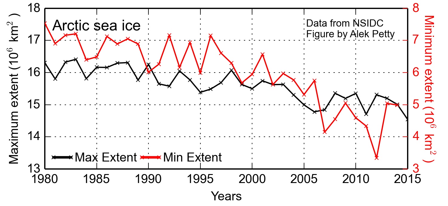
The summer Arctic sea ice minimum has decreased rapidly over the last several decades (see Figure 1). There has, however, been a well-reported increase in the sea ice minimum following the record low experienced in 2012 (also shown in Figure 1). This is not a recovery – the extent is still much lower than it was during the 1980s/1990s – but the surprising increase does suggest that our understanding of Arctic sea ice is far from complete. A post in this same blog series talked more about sea ice variability and the likelihood of such an increase, so I won’t say too much more on that.

This summer looks set to be one of the lowest minima on record. We still have a few days to go, but we probably won’t be witnessing a new record low unless something extremely drastic happens over the next few days.

Note that we tend to focus on summer sea ice extent as that’s when we see the biggest changes in Arctic sea ice. The maximum sea ice extent (which occurs in February/March) has still decreased over recent decades, but at a much lower rate. It’s going to take quite a shift in temperatures to stop most of the Arctic Ocean from freezing over in winter, although climate projections still show that could be a possibility in a century or two perhaps. A time series of the monthly Arctic sea ice extent is shown in the animation below.

The animation might fool you into thinking that there’s nothing to worry about, there’s still plenty of sea ice in the Arctic. But importantly, the thickness of the sea ice has reduced considerably over the same time period. Sea ice thickness is more of an ‘integrator’ of the atmospheric conditions than extent, and is therefore crucially important to those concerned with the changing volume of Arctic sea ice (plenty of scientists and stakeholders might in-fact be more interested in the location of the sea ice edge for various reasons too).

A recent study demonstrated a strong increase (~50%) in autumn sea ice volume after 2012, which they linked to a shorter melt season and the retention of older, thicker sea ice. Thickness might therefore be prone to considerable annual variability too. Again, this is by no means a recovery. Unfortunately, it’s a lot harder to measure sea ice thickness, so we tend to hear more about sea ice concentration/extent.

Sea ice models

To understand the physical mechanisms driving these changes, scientists often look to sea ice models – computer simulations of the sea ice cover.

Unfortunately, sea ice models have historically struggled to accurately simulate both the variability and long-term downward trend in Arctic sea ice extent. This was highlighted in the 2007 (AR4) Intergovernmental Panel on Climate Change (IPCC) report as a serious problem for the community, and serious efforts have been made to improve the accuracy of sea ice simulations in the years following.

Some of the processes included in the community sea ice model CICE – a popular, state-of-the-art, sea ice model developed in Los Alamos included in several global climate models – are shown in the diagram below. Note that some of these processes affect the sea ice thermodynamics (how the sea ice grows/melts), while others affect the dynamics (how the ice moves/deforms).

Even by 2007, sea ice models included several sophisticated parameterization schemes – a representation of some physical process that is too small or complex to be explicitly modeled – such as:

• Multiple ice thickness categories
• Multiple thermodynamic layers within the sea ice
• Brine storage (pockets of salt water within the ice)
• Sea ice rheology (how the ice moves/deforms under stress)

Upgrades were made to the sea ice models, and the 2012 IPCC (AR5) report showed considerable improvements in the simulation of the long-term decline. However, the simulations still showed wide spread across the various models. This was, and still is, a problem, as accurately representing sea ice in global climate models is important if we want to understand key physical processes taking place in the Arctic. The tele-connection between Arctic change and northern hemisphere weather patterns is just one of the important topics in our field where improved simulations of the Arctic sea ice state will result in increased understanding.

Improving sea ice models

So how do we improve sea ice models? For the most part, scientists focus on improving the physics of sea ice included within a sea ice model. The sea ice model physics is determined predominantly by the various parameterisation schemes included in the relevant sea ice model. We can therefore invest in improving the existing physics through calibration efforts (comparing with observations and tuning specific parameters), or we can add in new physics that was previously ignored/overlooked.

Since 2012, several new parameterisation schemes have been incorporated into sea ice models, including:

• Melt ponds (accumulation of melt water on the ice surface).
• Brine drainage through sea ice.
• Atmospheric/oceanic form drag (obstructions to air/water flow caused by the variable ice morphology).
• Anisotropic rheology (ice stresses in specific directions determined by ice floe shape).
• Lateral melt which accounts for variable sea ice floes.

To explain these sea ice model parameterisation additions more simply, I’ll provide a rather crude analogy. Sea ice models are a bit like an orchestra. The sea ice modeler is the conductor, each section (e.g. brass) represents a specific parameterisation scheme, and each musician represents a specific ‘free’ parameter within that scheme. The job of the conductor (sea ice modeller) is to ‘tune’ the musicians (parameters) to promote harmony (accuracy). Adding more musicians (parameters) or even sections (parameterisation schemes) gives us more instruments (parameters) to tune, making the job of keeping everything sounding good (accurate) somewhat more challenging. Increasing the instruments (parameters) available to ‘tune’ does, however, increase our overall level of control. A well-trained (calibrated) musician (parameter) will require less tuning. Adding sections (parameterisations) can be both a positive – through increased sophistication, and a negative – as there are more chances for the sound (model) to go drastically wrong. Pretty tenuous, but I think you get the gist.

Understanding Arctic sea ice melt variability

In a study published in the Proceedings of the Royal Society, led by my colleague Dr. Michel Tsamados, the CICE model was used to show that sea ice physics uncertainty might be significantly higher than previously thought. Essentially, various configurations of the new physics schemes cause a significant change in the simulation of the summer sea ice minimum. The lack of constraint of these new physics schemes with observations (calibration) is likely to be one significant reason for this uncertainty (adding in poorly trained musicians to our orchestra following the earlier analogy). It’s worth nothing also, that we are always going to be limited by the inherent uncertainty contained in climate models and the chaotic nature of the atmospheric/oceanic driving forces. We can, at least, lower the uncertainty caused by our own ignorance.

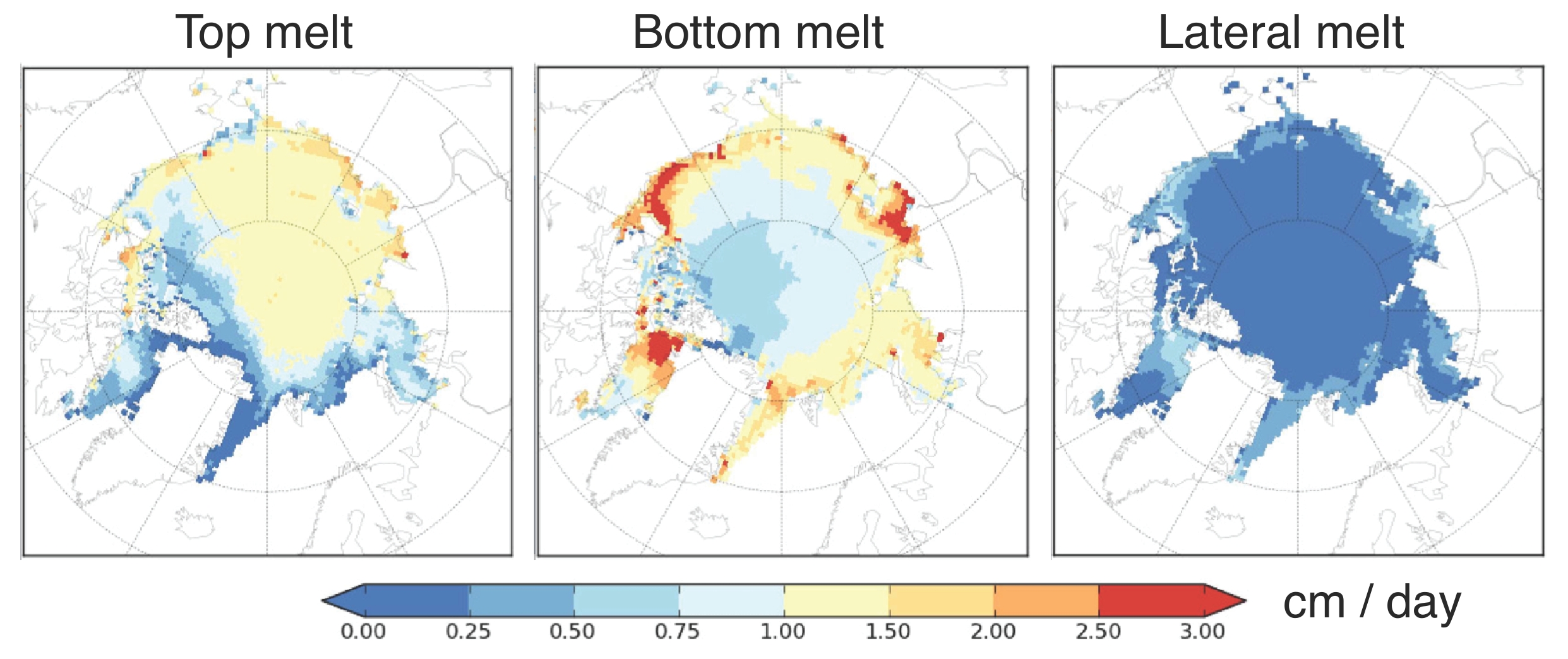
This new study also explored the impact on the sea ice melt season by looking at the contribution to the total sea ice melt from surface, lateral and bottom melting (see Figure 3). The simulations demonstrate greater variability in the surface melting of the sea ice cover (atmospheric driven) compared to bottom melting (ocean driven), despite bottom melt contributing more to the total melt. This might suggest that surface sea ice physics could be crucial in understanding annual variability. We’ll touch on this again in a bit.

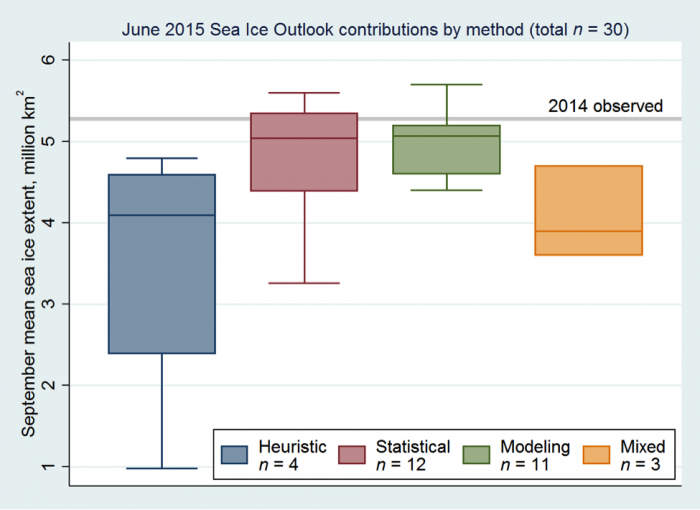
Another hot topic in the last few years has been sea ice prediction. This has mainly focused on the methods and our ability to predict the summer minimum extent, although there have been efforts to expand this to additional metrics of interest to the community (e.g. the likelihood of sea ice being present in a given location at a given time). The Sea Ice Prediction Network (SIPN) provides an open system for compiling and describing various predictions through their Sea Ice Outlook (SIO). The SIO monthly reports leading up to September (produced from June onwards) contain a variety of predictions based on estimates using statistical methods, climate model simulations, and ‘educated’ guesses (heuristic if we want to sound fancy).

It was recently shown that when the minimum extent followed the downward trend, the SIO predictions were pretty good, but when the extent deviated from this trend (anomalous years), the SIO predictions didn’t fare too well.

This could suggest that purely statistical and ‘heuristical’ methods of prediction might not cut it, as the physical forces contributing to each year’s melt season are so numerous and complex, that prior knowledge just won’t suffice. Predictions based on sea ice model outputs might, therefore, be our best bet. It’s worth noting also, that these models/predictions are never going to be perfect due to the inherent uncertainty in models and the climate system mentioned in the previous section.

My old colleagues at the Center for Polar Observation & Modelling (CPOM) made quite the splash a year or two ago when they produced skillful predictions of the Arctic sea ice minimum based on the simulated melt pond fraction in May (produced using the new melt pond scheme now included in CICE mentioned previously). The skill is thought to be due primarily to the positive albedo feedback mechanism – melting causes melt water to pool on the ice surface, which has a lower albedo than the ice (less sunlight is reflected away), leading to further heating, melting and ponding. More melt ponds in spring should therefore result in more melting of the sea ice cover through the melt season. This was discussed on this blog a year back, so do check out that link for more information.

The median prediction from this year’s June Sea Ice Outlook (5.0 million km²) looks to be on the high side, as the extent creeps towards 4 million km² with a few days of melt still to go. Clearly our understanding of Arctic sea ice is still lacking.

Final thought

So, sea ice models – they can’t reliably predict or simulate the Arctic sea ice cover, but they could, and indeed they should. Improved sea ice physics and the calibration of existing physics with observations are urgently needed for all those interested in Arctic and indeed global climate. Huge advances have been made in recent years, but there is still some way to go before we can reliable simulate and predict the fate of the Arctic sea ice cover.

Alek (@AlekPetty)

p.s. I didn’t even mention Antarctic sea ice. We can talk about that in six months time…!