Often when analysing and comparing climate data we have to choose a reference period (or baseline) to calculate anomalies. But it is not often discussed why a particular baseline is chosen. Our new paper (open access in BAMS) considers this issue and asks: does the choice of reference period matter?
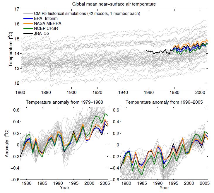
Consider simulations and reanalyses of global mean temperature, without using anomalies (Fig. 1). Each climate model has a different value for global mean temperature (with a min-max range of about 3K), but all show similar changes over the historical period (grey). The range amongst the different reanalyses (based on assimilating observations) is about 0.5K, highlighting that is difficult to estimate the real world global mean temperature precisely (colours). To compare the simulated changes with those from reanalyses, a common reference period is therefore needed.
Two immediate questions arise: do these differences in mean temperature matter? And, does the choice of reference period matter?
Do these differences in global mean temperature matter?
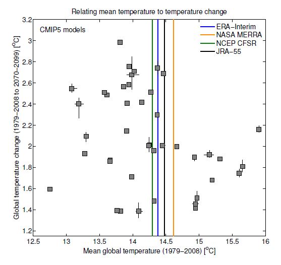
Fig. 2 shows that future changes in global mean temperature are not strongly related to the simulated global mean temperature in the past – there is no robust correlation between the two, and there are good physical arguments for this (see Appendix A in Hawkins & Sutton, or this RealClimate post).
Does the choice of reference period matter?
Short answer: yes. The lower panels in Fig. 1 show the same data as anomalies, using two different but equally valid choices of reference period. Note that the impression of where the reanalyses fall within the model range is markedly different when making the two choices. You might draw different conclusions based on the left or right panel only.
The choice of reference period also matters when assessing expected changes in global mean temperature over the next couple of decades, and for assessing when the 2°C above ‘pre-industrial’ global temperature level might be reached. These examples are discussed in detail in Hawkins & Sutton, but here we use an analogy instead.
Different time series can be thought of as stiff (and “wiggly”) wires that are required to pass through a fixed length of tube. Different length reference periods correspond to tubes of different lengths, with longer tubes required to have wider diameters. There is little constraint on how the wires spread outside the tube, and for longer tubes, less constraint on how they vary within the tube, thanks to a larger diameter. In the extreme, a tube that is one time point long would have zero diameter because all of the wires can be forced to pass through the same point. The constraint on where the wires are positioned vertically, relative to each other and relative to the tube, varies as the tube is slid horizontally along the loose bundle of wires.
Interpreting the wires as time-series of annual mean global mean temperature illustrates the effect of choosing a reference period. Which is the warmest timeseries at later times depends on the choice of reference period (or tube position). The black dashed lines show the range of possible futures for a larger set of time-series demonstrating that the uncertainty shrinks for later reference periods.
Overall, there is no perfect choice of reference period. A strong recommendation is that any studies that seek to draw quantitative conclusions from analyses that involve use of a reference period should explicitly examine the robustness of those conclusions to alternative choices of reference period.
Paper: Hawkins & Sutton, Connecting climate model projections of global temperature with the real world, BAMS, in press (open access)
[Thanks to Francis Zwiers for suggesting the wire analogy.]
Nice artcle, the wire demo/tube is great.
Does baselining cause an artificial reduction in the spread of the model runs immediately before and after the end of the baselining period as a result of auto-correlated sources of natural variability (e.g. modelled ENSO)? I noticed suggestions of this while experimenting with model-obs comparisons, but didn’t get round to studying it properly. My intuition is that if there are medium term unforced quasi-periodic components that are long enough not to completely cancel out over the course of the baseline period, then they will affect the baseline adjustment and this adjustment will continue to have a small effect outside of the window because of the autocorrellation.
I probably haven’t described that very well, but it concerned me that it may be a source of bias that increases the chance of detecting a spurious model-obs inconsistency (less important that the issue presented above and e.g. other issues).
Yes – I agree that there probably is an influence just outside the choice of reference period due to auto-correlation as you suggest, but I think in most cases this will be a small effect.
Thanks,
Ed.
The models have a 3°C spread in absolute temperature. Absolute temps are important in a number of physical processes such as freezing/melting and condensation.
Has anyone looked at the effect this has on modeling climate?
Hi Robert,
Good question – the full paper discusses this point. For global temperatures, it doesn’t seem to make much difference. On regional scales, this is less clear due to the physical processes associated with phase transitions, as you say. More work needed to examine this!
Ed.
This is a great analysis. I particularly like this statement in the paper.
It may be a surprise to some readers that an accurate simulation of global mean temperature is not necessarily an essential pre-requisite for accurate global temperature projections.
While this is certainly true for measurements, I am a little surprised at the wide spread of model results for absolute temperature. Since 70% of the surface is ocean much of this average of up to 3 degree difference must be in SST. Individual grid cell T-differences must be much higher.
How are models initialised? Is the surface temperature just an emergent result from inputs of TSI, ice, topology, atmospheric content, vegetation, ocean circulation etc? Or do they start with an intial temperature field?
Is the time step for CMIP5 days or hours ?
Hi Clive,
Almost everything is emergent in the CMIP5 simulations! The fixed inputs are topography, land-sea mask etc. The time varying inputs are atmospheric concentrations, land cover type, TSI, orbital parameters, volcanoes etc. The ocean circulation, ice, temperature etc are all emergent. There is obviously an input initial state to start the simulation, but the model is run for several hundred years to ensure it is stable before any of the historical simulations are started, and the initial state is irrelevant.
The time-steps are typically of the order of an hour or so. The high-resolution simulations have time-steps of few minutes.
Ed.
No that’s not what all CMIP exercises do. Many, especially within the exercises which start from 1960, are REINITIALIZED, (RESET in other words) with observed values every 5 years. If that is not done, then the model temperature results rise like balloons to unbelievable temperatures.
CMIP, as some sort of validation of the skill of the gcms for long term forecasting, is a spurious sham, if I’m not mistaken.
Ed, how much detail can you supply into the dynamic of model emergent ENSO? I realize this is a relatively new feature in GCMs. Does ENSO emerge like I presume volcanoes would, by a random generator, or do oscillations gradually form, or is there an oscillation underway at every particular time point, like a continually running sine wave?
Hi Ron,
ENSO is not a new feature of GCMs – they have been simulating it since the earliest models were written. And, it emerges naturally from the physical laws on which the models are based. There are no stochastic random generators, or input sine waves. Volcanoes are prescribed to occur at the observed time in simulations of the past and there are no volcanic eruptions in future simulations.
Ed.
Ed, I have also looked into this ENSO feature of CMIP and I couldn’t find any mention in any document of ENSO being accurately simulated as ’emergent’. Rather, by reading the references below, I learned, again, that ENSO is not accurately simulated at all. Rather it is a parameter that is continually reset in order to prevent the modeled temperatures from rising like balloons into unbelievable values. References follow. I’m interested to get to the bottom of this, so if you have a reference to back up your statement, please post it soon.
Radic´, V. and G. K.C. Clarke, 2011, Evaluation of IPCC Models’ Performance in Simulating Late-Twentieth-Century Climatologies and Weather Patterns over North America, JOURNAL OF CLIMATE, American Meteorological Society. DOI: 10.1175/JCLI-D-11-00011.1
http://journals.ametsoc.org/doi/abs/10.1175/JCLI-D-11-00011.1
Here’s a gem, as the title suggests something quite opposite to the actual paper content.
5d: Gonzalez, P.L.M,and L. Goddard, 2015, Long-lead ENSO predictability from CMIP5 decadal hindcasts. Journal of Climate Dynamics DOI 10.1007/s00382-015-2757-0
this reference is a little more candid
Kharin, V.V., G.J. Boer, W.J. Merryfield, JF Scinocca, and W.S. Lee, 2015, Statistical adjustment of decadal predictions in a changing climate GEOPHYSICAL RESEARCH LETTERS, VOL. ???, XXXX, DOI:10.1029/, downloaded from jcli-d-11-00011%2E1.pdf
this reference is especially pertinent, and about as candid as such critiques have ever reached to date.
Fricker, T.E., C.A.T. Ferro, and D.B. Stephenson, 2013, Three recommendations for evaluating climate predictions METEOROLOGICAL APPLICATIONS 20: 246 – 255 DOI: 10.1002/met.1409
Hi Michael,
You can read about the CMIP5 experimental design here:
http://journals.ametsoc.org/doi/abs/10.1175/BAMS-D-11-00094.1
There are different sets of simulations in CMIP5 – the vast majority of which are NOT reinitialised. These are the ones used in all the projections you will usually see. There are a subset which are experimental decadal predictions which are reinitialised every year from 1960 onwards – these are only used in part of Chapter 11 of IPCC and not in any of the Summary for Policymakers figures.
See this paper for ENSO simulations in CMIP3 and CMIP5:
http://link.springer.com/article/10.1007/s00382-013-1783-z
CMIP is not a spurious sham – you are mistaken. The temperatures are projected to rise, but not to unbelievable values. The GCMs are based on the fundamental physics of the atmosphere and oceans etc. The greenhouse effect has been known and understood since the 1860s.
cheers,
Ed.
Ed, this is very funny, or would be if the stakes were not so high.
As you know Chapter 11 of IPCC is all about assessments of the predictability skill of your models. And buried in that assessment are such statements as “In current results, observation-based initialization is the dominant contributor to the skill of predictions of annual”
In other words, I am right, the models can’t predict squat.
Thanks for the paywalled reference, I’ll read with interest.
In the meantime, here is a link to my own industry study, a less expensive item at
http://www.abeqas.com/the-most-transparently-accurate-climate-forecasts-in-the-world/
Hi Michael,
I believe your statements are based on a fundamental misunderstanding of what the various sets of simulations are designed to do.
The normal uninitialised projections are designed to project the long-term climate effects of changes in greenhouse gases, solar activity, aerosols, volcanic eruptions etc. They are NOT designed to forecast the year-to-year variations of the climate. However, being based on the laws of physics, these simulations produce those variations in climate (e.g. El Nino, AMO, PDO etc), but not necessarily at the same time as the real world.
The initialised experimental decadal predictions are designed to predict some of the year-to-year fluctuations, as well as any trend – hence the statement in Chapter 11 about being able to predict the climate a year ahead relies more on the variability than the long-term trend.
cheers,
Ed.
The ’emergent ENSO’ is just what ’emergent’ means, that is, there are no additional functions for creating ENSO in sophisticated models, but the ENSOs in these models emerge by normal flow functions. Ed might clarify. I would imagine someone working on these might be offended if someone suggested adding a separate function for this, and indeed they have (asked about this on RC sometime in 2009).
On to the subject in hand, a proper baseline might be obtained from the pre-industrial runs on the more accurate models, this however, likely leaves out some of the mods humans have done on wild vegetation, as there are still preciously few models on climate and agriculture/forestry.
If the object of a baseline is to have a fixed reference upon which variation can be compared I agree a modeled baseline with all parameters arbitrarily fixed at the best estimated values would be the solution. Is there a possibility there could be a consensus on the best parameters and the best model? That I would guess is a harder problem.
It sounds like you’re referring to an approach that’s already being done, although perhaps not systematically.
For example, climate models simulate the formation of rainfall in different ways and have various parameters, such as a “critical radius” above which rain drops start to fall. It’s crazy hard to do lab tests on this because you need real-world conditions. So people have been combining satellite measurements to try and get at this – such as using MODIS which can estimate droplet size with the Cloudsat radar that tells you whether rain is falling.
http://journals.ametsoc.org/doi/abs/10.1175/2010JAS3463.1
From this you can work out what certain parameters should be.
Unfortunately, there are so many competing factors in the models that it’s still very difficult to untangle all of them. One might be better at doing rain but if you take its parameters as being the “best” and apply them then maybe you screw up the humidity in the subtropics (random example I just made up).
I think you’re right about it being a hard problem Ron!
When I said “best” I really meant two factors for each parameter to consider. The first which would be the the most optimal value, the second being the most validated accuracy. To gain the first I would choose the most important parameters that have known optimums and them derive and calibrate the other parameters off this backbone. And it this produces the best target climate, that should become the standard upon which others are judged. I presume, for example, a GMST somewhere between that of the 1890s and 1920s would be considered optimal.
As I understand it, there are too many possible combinations of parameters that give the “right” answer for us to be sure. Work is being done to rule out as many combinations as possible but I don’t believe this is going to be solved any time soon… there are papers comparing projected changes versus known current conditions, this being a typical “emergent constraints” method that’s kind of similar to what you’re suggesting. Iirc so far this technique has generally found that models that do a better job of matching various observed properties tend to be on the higher end of the climate sensitivity range, for example.
If you’ve got a suggestion about how to pick the “most important” parameters objectively and efficiently then I guess a lot of researchers would be pretty excited about it.
Also – we don’t know the global mean temperature precisely now, nevermind back in 1900 (see the figure in the post)!
As the full paper discusses, the most important aspect of a GCM to get right is the energy balance, rather than GMST.
Ed.
“If you’ve got a suggestion about how to pick the “most important” parameters objectively and efficiently then I guess a lot of researchers would be pretty excited about it.”
It would make everyone uneasy but a multi-blind trial is the best way to quash favoritism. The first blind would be anonymous polling for the best methods to set criteria for a trial. The second blind would be the running of the models and evaluation of output. The final conclusions would also be from a blind vote. This one consensus that would be mostly accepted, including by outsiders on all sides.
To get at energy balance and optimal GMST I would include in the project all a hard sciences involved in climate to establish a blind consensus on ocean temp, TOA imbalance, cloud and precip trends from all sides remote sensing to paleo. I know it’s improbable but what is optimal was the question. I’m curious what others think.
Ed,
I have been looking in detail at the geographic difference in surface temperatures between CMIP5 models. A ‘warm’ model such as GFDL-CM3 has a completely different temperature map than a ‘cooler’ model such as GISS-E2-R. The largest differences are in the Arctic, Himalayas, Andes and central Africa. This is consistent throughout the projections with the Arctic discrepency of over 5C spreading in extent throughout Russia and Canada by 2100.
There seems to be a gentleman’s agreement among modeling groups not to criticise other members of the CMIP5 ensemble. I understand that huge amounts of effort is put into developing each GCM, but they simply can’t all be correct.
Physics has always been based on developing theoretical models to describe nature. These models make predictions which can then be tested by experiment. If the results of these experiments dissagree with the predictions then either the model can be updated to explain the new data, or else discarded.
Surely we are at the stage that we can distinguish between models based on measurements. Why is this not being done?
Hi Clive,
Yes – the models do show large regional differences in temperature. There are numerous publications which try and rank models by performance, so I think there is such criticism.
It is not (yet) possible to build a complex GCM which matches observed estimates of every variable – decisions are made about which aspects of climate to prioritise getting ‘right’. In some cases, it has been subsequently found that the observations were biased, and this has been identified because the GCMs disagreed with the observations.
Model developers are aiming for what you suggest, but it is not always possible. Partly this is because these models take so long to run, that only a finite number of changes can be tested on each development cycle.
cheers,
Ed.
I believe it is not being done because the train has left the station Clive.
Does the train have a driver or any brakes?
An interesting article, Ed..
However, I am not astonished that the models produce global absolute temperatures on quite different levels. I have looked into TOA imbalance of CMIP5 models recently, and found that the sun radiation reaching TOA (rsdt) differed with more than 3 W/m2 between different models.
This spread in rsdt is not very realistic. From satellite measurements the TSI can be accurately determined, and in the future some kind of 11-year cycles could be assumed. IPCC should provide a “fixed” rsdt-scenario to be used by all models ( just like the rcp:s). I believe that this would reduce the spread in absolute global temperatures among models..
Concerning the reference periods I believe that, if possible, the best choice is a 60-year base period. According to the temperature records, there seems to be some kind of 60-year cycles involved, altering the distribution of ENSO, etc. With a 60 year base those ups and downs would be equalled out. Since the temperature record before 1946 is less reliable the best choice of normal period should be 1951-2010.
Btw, My interest in TOA imbalance was a crude test of models vs observations in global heat accumulation. Yes, I trust the models, at least the average of all models which is seemingly spot on: 13.3 vs 13.4*10^22 J accumulated heat during the Argo era.
https://drive.google.com/file/d/0B_dL1shkWewaaWtldTV6TTktSDQ/view?usp=docslist_api
Credits to KNMI Climate Explorer…
Hi Olof,
My understanding is that the absolute value of TSI is not known that precisely – see, for example, which also has a ~3W/m2 spread for observations:
http://www.acrim.com/
Would be interesting to see if the high TSI models have high GMST as well? The 11-year solar cycles as observed are used up to 2005, and then a repeating 11-year cycle is assumed thereafter in the CMIP5 simulations. I agree it might make sense to fix TSI across simulations.
As for reference periods – using a long period is helpful, but we don’t always have data for 60 years. For many applications we only have data since 1979 for example.
cheers,
Ed.
Thanks Ed,
I wasn’t aware of the uncertainty in the TSI measurements, but after You mentioned it I actually noticed in KNMI climate explorer that it is a reconstructed value, with a link to a paper http://www.pmodwrc.ch/pmod.php?topic=tsi/composite/SolarConstant
Figure 2 show three reconstructions, PMOD composite and ACRIM composite have an average TSI of about 1366 W/m2 whereas the IRMB composite run 4 W lower. Divided by four this gives a difference in rsdt of about 1W.
As I remember, a majority of the models had an rsdt of about 341.5 W/m2 so they likely followed the 1366 W/m2 composites above.
Almost all models follow near 11-year cycles in the future, but with time the cycles get more and more out of sync.
If there is a real uncertainty in the actual level of TSI, it can be motivated to run the models on different levels of rsdt, e.g. by IPCC regulated high, middle and low scenarios, but I guess that they don’t have to be more than plus/minus 1 W apart .
AFAIK the latest value of TSI is 1360.8 ± 0.5 W/m-2 at solar minimum (ref. Kopp & Lean 2011), which is considerably lower than the canonical value canonical value of 1365.4 ± 1.3 W m−2 , and corresponds with an effective solar temperature of 5770 K. So if some models are still using the older value this might explain some of the difference.
Ed, regarding TOA imbalance, how prevalent is the assumption of TOA steady-state as being in the pre-industrial era, 1800-1860? I ask because the Oceans2K paper published in August shows a steady decline in SST over the past 2K years in a comprehensive multi-proxy study. But the MWP did not even register a signal, and strangely, neither did the modern warming period. Many are scratching their heads but is a possible explanation that the ocean temps have been lagging a 2K-yr decline in GMST, and thus the steady-state TOA was only reached in the 20th century while GMST had swung up to meet SST’s lag?
https://climateaudit.files.wordpress.com/2015/09/high_resolution.png
Also, the authors claimed most all of the cooling to be correlated to volcanic activity, which the authors claimed was successful validated in a GCM.
http://www.pages-igbp.org/ini/wg/ocean2k/nature-geoscience-2015-faqs
Are you familiar with this and is there potential for more cross-validation of GCM’s with good paleo studies?
Hi Ron,
The models tend to be developed in a pre-industrial control simulation where forcings are fixed at ~1850 levels. The developers aim for a TOA balance in those simulations, before starting the historical simulations. Not very knowledgeable on the paleo studies, including the Oceans2K one, but lots of papers which test GCMs in past climates, e.g. Last Glacial Maximum, and compare with available proxy data.
cheers,
Ed.
Hi Ed,
The assumption that the real climate was in equilibrium immediately prior to the start of the historical simulations in 1850 or 1860, as is assumed for the CMIP5 historical simulations, seems very doubtful. The Earth was still recovering from the Little Ice Age (largely volcanic driven according to model simualtions, IIRC) at that time. The past1000 year (850-1849) CMIP5 simulations show aTOA imbalance in the 1820s and 1840s (volcano free decades) of ~+0.2 W/m2 relative to their preindustrial control runs. The problem of omitted pre-1850 volcanic forcing biasing 1850-on simulations was highlighted in Jonathan Gregory’s 2013 GRL paper ‘Climate models without pre-industrial volcanic forcing underestimate historical ocean thermal expansion’ (implying that they have a downwards bias in their historical period simulated ocean heat uptake).
Hi Nic,
Yes – I agree it would be ideal to start the pre-industrial / historical simulations earlier. Obviously there is a bit of a compromise because of computational cost, but 1750 would be better, which is after the Little Ice Age (Maunder Minimum and some eruptions) but before the early 1800s eruptions and Dalton Minimum. [Actually working on a paper which will make such a recommendation.]
cheers,
Ed.
Sorry for the slight off topic.
– Volcanoes are prescribed to occur at the observed time in simulations of the past and there are no volcanic eruptions in future simulations.
Is there any rough estimation of the difference on the model’s warming of the past with and without volcanoes? Say, the difference of model’s temperature in year 2000, with and without volcanoes? Or maybe it doesn’t make a relevant difference.
Hi plazaeme,
Global temperatures would be warmer than they are now without the volcanic eruptions, but it is not clear how much. Probably less than 0.2K.
There are simulations done just with volcanic and solar changes which help look at this, e.g. see Figure 10.1 of IPCC AR5 WG1.
cheers,
Ed.
Thank you very much.
Ed,
Is that really true? The volcanic dust from Mount Pinatubu in 1991 cooled the earth by about 0.35C lasting between 1-2 years. The dust had cleared by 3 years after the erruption and temperatures returned to normal. Volcanoes do not have any long lasting effect.
I suppose there might be some low level dust from small volcanoes errupting continuously, and this would then vary strongly with volcanic activity. This was also the Nuclear Winter scenario where a nuclear war floods the startosphere with dust causing a new Ice Age.
Hi Clive,
One example of a long volcanic response is here:
http://journals.ametsoc.org/doi/full/10.1175/2011JCLI4067.1
Impacts on ocean heat content (and sea level).
cheers,
Ed.
Drat! Its those damn oceans again !
cheers
Clive
My question revolves around the idea that one can graph the model ensemble data and obs data and make comments on the extent to which they match/diverge and for that to have any great meaning.
Given that
The baseline period is usually 1961-1990 that gives us 25years for the two datasets to develop.
Expectations are around 0.2degrees per decade increase in GMT from forcings. About 0.5degrees in 25years.
Ensemble model spread is roughly around 0.5degrees or more ATM.
Year to year changes in the obs GMT can be as high as 0.5degrees or more.
The chances that these two datasets are going to diverge in such a short period of time given some of the statistical properties of the datasets look remote. You could also nuance the problem even further given that the more interesting climate discussion isnt so binary as warming or not but the rate of warming. For example we are told people who are apparently on different sides of the discussion over TCR are probably really arguing about whether the forced rate of change is ATM 0.1oC or less compared with 0.2oC or more. In this case whether model ensembles statistically match obs or not would seem irrelevant.
I have a few further points . The second part of figure 2 is an interesting example about how images can convey meaning. You show only 1980 onwards in those graphs. Anybody looking at those might think models are doing a great job matching obs. But part of the data includes the baselined period in which statistical processing has forced the data to match and we only have a couple of decades for the two datasets to wander. The really wonky stuff is back in the early 20th century, well thats what your neat final animation would suggest.
Anyway great post, the final animation is a really neat way of visualizing the issue.
Very nice animation showing the influence of the baseline period. This is relevant to the case of Spencer using a very short and early baseline when comparing models to satellite temperatures, which by virtue of his choice of baseline inflates the appearance of a discrepancy. See e.g. https://ourchangingclimate.wordpress.com/2014/02/22/john-christy-richard-mcnider-roy-spencer-flat-earth-hot-spot-figure-baseline/