Climate sensitivity characterises the response of the climate to changes in radiative forcing and can be measured in many different ways. However, estimates derived from observations of historical global temperatures have tended to be lower than those suggested by state-of-the-art climate simulators. Are the models too sensitive?
A new study largely explains the difference – it is because the comparison has not been done ‘like-with-like’.
The implications for understanding historical global temperature change are also significant. It is suggested that changes in global air temperature are actually ~24% larger than measured by the HadCRUT4 global temperature dataset.
Post based on Richardson et al. (2016, Nature Climate Change) [code & data]
Historical weather observations include air temperatures measured over land areas and sea surface temperatures in ocean regions, but only where there were existing thermometers (& ships). The observed change in ‘global mean temperature’ is produced by blending together these sparse, differently measured changes of temperature over time (e.g. for HadCRUT4).
However, when considering global mean temperature from climate models, we tend to use simulated air temperatures everywhere, mainly because this is much easier to calculate. Does this difference matter?
An earlier study by Cowtan et al. demonstrated that these subtle differences in producing estimates of global temperature can make a significant difference to conclusions drawn from comparisons of observations and simulations.
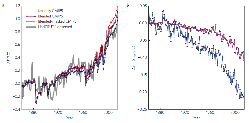
As we cannot travel back in time to take additional historical observations, the only way to perform a like-with-like comparison is by treating the models differently, in terms of the spatial coverage and observation type. Figure 1 highlights the dual effects of ‘masking’ the simulations to have the same spatial coverage as the observations and ‘blending’ the simulated air and sea temperatures together, instead of using air temperature everywhere.
When using simulated air temperatures everywhere (Fig. 1a, red line), the models tend to show more warming than the observations (HadCRUT4, grey). However, when the comparison is performed fairly, this difference disappears (blue). Roughly half of the difference is due to masking and half due to blending.
The size of the effect is not trivial. According to the CMIP5 simulations, more than 0.2°C of global air temperature change has been ‘hidden’ due to our incomplete observations and use of historical sea surface temperatures (Fig. 1b).
But what effect does this have on estimates of climate sensitivity?
Otto et al. (2013) used global temperature observations and a simple energy-budget approach to estimate the transient climate response (TCR) as 1.3K (range, 0.9-2.0K), which is at the lower end of the IPCC AR5 assessed range (1.0-2.5K).
A new study, led by Mark Richardson, repeated the analysis of Otto et al. but used updated observations, improved uncertainty estimates of aerosol radiative forcing and, critically, considered the blending and masking effects described above.
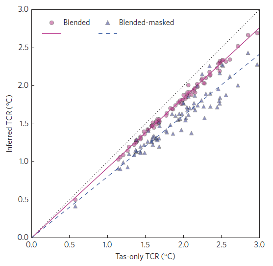
Figure 2 shows how TCR estimates from different CMIP5 models depend on the assumptions made about observation availability. The pink circles highlight that the blending procedure lowers the TCR when compared to using air temperature (tas) everywhere (dotted black line). The blue triangles demonstrate that the sparse availability of observations further reduces the TCR estimates.
So, according to the CMIP5 simulations, the TCR estimated from our available observations will always be lower than if we had full spatial coverage of global near-surface air temperature.
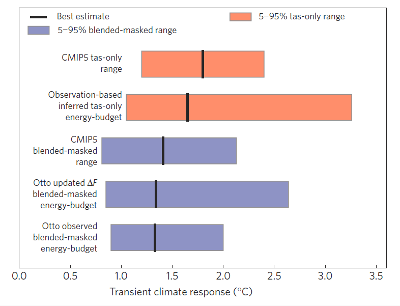
To summarise the effect of the differences in analysis methodology, Figure 3 shows various estimates of TCR. The top red bar shows the raw estimates of TCR from the CMIP5 simulations and the bottom blue bar is the original result from Otto et al. based on observations. The various bars inbetween reconcile the difference between Otto et al. and CMIP5.
For example, if the models are treated in the same way as the observations, then the estimated TCR is the top blue bar, in much better agreement with Otto et al. There is then no discrepency between the observation and simulation estimates of TCR when they are treated the same way. (The second blue bar shows the impact of updating the uncertainty estimates of aerosol radiative forcing on the Otto et al result, which is a separate issue.)
However, we can also reverse the procedure above and estimate by how much we need to scale the TCR estimated from the observations to reproduce what would be derived if we had air temperatures everywhere. This is the second red bar in Figure 3, which overlaps the CMIP5 simulation range and has a best estimate of 1.7K (range, 1.0-3.3K).
Richardson et al conclude that previous analyses which reported observation-based estimates of TCR toward the low end of the model range did so largely because of inconsistencies between the temperature reconstruction methods in models and observations.
As observational coverage improves the masking effect will reduce in importance but will still remain for the historical period unless we can rescue additional, currently undigitised, weather observations. The blending issue is here to stay unless estimates of changes in air temperature can be produced over the ocean regions. The physical mechanisms for the different simulated warming rates between ocean and air temperatures also need to be further explored.
Finally, if the reported air-ocean warming and masking differences are robust, then which global mean temperature is relevant for informing policy? As observed? Or what those observations imply for ‘true’ global near-surface air temperature change? If it is decided that climate targets refer to the latter, then the warming is actually 24% (9-40%) larger than reported by HadCRUT4.
And that is a big difference, especially when considering lower global temperature targets.
What are the results using datasets with more sensible interpolation schemes than HadCRUT4, eg GISTEMP?
Hi GJ – think one of the co-authors is working on that aspect. The ~10% blending issue will still be there I suspect. Ed.
Geert Jan van Oldenborgh,
It depends a bit on time period and calculation. Using datasets beginning in the 1860s (HADCRUT4, Cowtan and Way, BEST) with the one-box (e.g. Held et al., 2010), difference (e.g. Otto et al., 2013)
Method HadCRUT4 CW BEST
Onebox 1.48 1.57 1.61
Difference 1.34 1.45 1.42
Trend 1.17 1.23 1.17
(note: “trend” uses 1970 onwards and in models underestimates their true TCR, because TCR is defined over 70 years. Model TCR is about 20% higher than you get if you apply the trend method to each model and it’s more sensitive to changes in recent forcing or variability. Would be interesting to see what England et al.’s results mean for this)
Starting in 1880 to include GISTemp:
HadCRUT CW BEST GISTemp
Diff 1.20 1.31 1.4 1.25
Onebox 1.45 1.53 1.59 1.55
Trend 1.17 1.23 1.17 1.19
Our supplementary information shows that the result depends on time period also in models, for no time period does the difference result fall below the 20th percentile or above the 80th percentile of the models iirc.
Direct comparisons with GISTemp are harder as we haven’t implemented a “GISTemp simulator” for models. There’s also some weird stuff going on near WWII in some of the SST records which has a different effect in HadSST and ERSST. The best we can say right now is that the energy balance approach doesn’t really give strong evidence for lower TCR than the models give.
Wouldn’t we expect a larger change in the beginning of the 20th century, when the Arctic was warming strongly, which is a region where we do not have much observations? Or was this warming unforced (or still unexplained) and not in the models?
Hi Victor,
The right panel of Figure 1 tries to help us look for stuff like this. The difference between blue and magenta is the masking effect, make of that what you will.
Kevin Cowtan’s site contains .nc files of each model’s temperature maps by year for each reconstruction method if you want to do anything fancier. That’s in his site for his last paper on reconstructions. The one linked by Ed contains the annual time series.
As far as I can tell this analysis uses the same Kevin Cowtan’s result from the ‘Apples to Apples’ paper. I found that up to 2015 the ‘blending’ bias with H4 was only about 0.05C.
http://clivebest.com/blog/?p=6788
Therefore I presume the higher new estimate for TCR is because it now includes the later ‘El Nino’ enhanced date for 2016. Therefore you should repeat the analysis in 1 years time to get a more representative sample.
Clive: Is it a baseline issue? Mark is using a 1861-1880 baseline for comparison to Otto et al. In the rcp85-xax runs I see 2014 at about 0.09C above 1861-1880.
Hi Clive,
Supplementary Info contains tables for different start and end dates. We weren’t able to push past 2010 because we needed a year-by-year forcing series to do the one-box and trend calculations, and for obs we only had the Otto forcing as a published year-by-year series that was easy to work with.
In our paper “blending” refers to Cowtan et al.’s “xax”. Sea ice retreat enhances the blending effect, which is explained in the supplementary information to Kevin Cowtan’s paper. Arctic sea ice changes dominate Antarctic because we have better coverage there than in the southern ocean.
Extending to 2015 and using more modern forcing (e.g. from Schmidt) would probably slightly boost our observational TCR estimates.
IMO evidence on recent variability favours higher obs estimates, evidence on aerosols points lower and WWII SST or southern ocean changes could depend on the dataset. We provide large uncertainty ranges but for now I don’t think there’s any good evidence that the energy budget suggests lower TCR than models to any practical extent. Previously it could be argued that although they didn’t lie outside the model range, in a Bayesian sense they could notably shift our best estimate.
Wonder if this study accounted for lower recent F than used in CMIP5 per Schmidt et. al. (2014) or higher aerosol forcing efficacy per Marvel et. al. (2015). If not, then a further upward adjustment in the “observational-based” energy-balance TCR may be needed.
Hi Chubbs,
We did not, both of those would favour slightly higher TCR but the effect of the Schmidt forcing shouldn’t be too big because we’re looking long term, with total forcing changes of about 1.94 W m-2. Schmidt’s forcing is more relevant for shorter-term calculations.
We wanted to allow a direct comparison with Otto (and partly Lewis and Curry) which explains our approach. Results might change again in the future, we’re not at the end of this yet!
Thanks for writing this Ed. I don’t have any comment on the paper itself (mainly because I don’t have it) but rather on Kyle Armour’s News and Views piece, which discusses the paper in the larger context of the conclusions drawn by Marvel et al. and a set of five referenced papers that he claims address the issue of a mismatch between what early observations indicate for ECS, where he states, near the end:
“Although observation-based studies make the implicit assumption that climate sensitivity estimated today will still apply in the distant future, a recent line of research [refs 7-11] calls this into question based on a robust behavior of climate models–in the early warming phase, climate sensitivity appears smaller than its true value. This requires yet another upward revision to observation-based estimates (by around 25% on average) in order to achieve an apples-to-apples comparison with models.”
I don’t understand this statement at all. Aside from the fact that attempting to estimate ECS from a few decades of observations is inherently very problematic due to the very different time scales involved in each, it seems clear to me that the model-based analyses of Gregory, Goode, etc., and especially Caldeira and Myhrvold (2013) indicate that observations of a climate system undergoing a strong and consistent RF increase–say a 1% per year CO2 increase–indicate unrealistically high rates of warming in the first few decades, which then taper off drastically later, leading to a long but gradual climb to the ECS temperature (the “slow” component of forced warming, to use I. Held’s phrasing). So I have no idea what Armour is referring to there.
Of course, that’s a comment/question for him and I don’t expect you to know exactly what he meant, although if you have thoughts on the matter, fire away by all means.
Armour reference:
http://www.nature.com/articles/nclimate3079.epdf?author_access_token=LNQKgwEONy5YVJSvlubB29RgN0jAjWel9jnR3ZoTv0PPTNF_sOIeFx9myJ_U10XLsj8_p1lqjx0RRDTJbTTc78eupvudlmNtEiNXnWHNhr4crt8ZuOmLA66TNpMu_PUg
I have to re-phrase what I said above because it’s not what I meant to imply: replace “unrealistically high rates of warming in the first few decades” with “high rates of warming in the first couple of decades which then decrease over time”. These two rates correspond to the fast and slow rates described by Held and quantified by Caldeira and Myhrvold (2013) for all CMIP5 GCMS, using 2- and 3-parameter exponential models.
Hi Jim,
Not had time to read the Armour commentary in detail yet – but it sounds like he may be referring to the ‘cold start’ problem? http://link.springer.com/article/10.1007/s003820050201
Also – ECS will also change with base state due to changes in the feedbacks (e.g. albedo), i.e. if you double from 1x to 2x CO2, the warming may be different to going from 2x to 4x even if the forcing is the same.
cheers,
Ed.
Hi Jim and Ed,
What I was referring to in the News & Views was the fact that nearly all GCMs show global radiative feedbacks changing over time under forcing, with effective climate sensitivity increasing as equilibrium is approached. As a result, climate sensitivity estimated from transient warming appears smaller than the true value of ECS. This effect has received a lot of attention recently (see papers I referenced, and many more cited therein), and my intention was to show how it compounds with the results of Richardson et al and Marvel et al. If nature behaves similarly to the models, those observation-based estimates of ECS have to be increased by another 20-30% or so (some GCMs suggest much more than this, and others a little less).
As far as we can tell, the physical reason for this effect is that the global feedback depends on the spatial pattern of surface warming, which changes over time. In particular, the pattern of warming in the first few decades is distinct from the pattern of warming in equilibrium, so the global radiative feedback and effective climate sensitivity are distinct as well. One nice example is the sea-ice albedo feedback in the Southern Ocean: because warming has yet to emerge there, that positive (destabilizing) feedback has yet to be activated; but it will be activated eventually as the Southern Ocean warms over the next several centuries, leading to higher global climate sensitivity. And tropical cloud feedbacks appear to depend on the pattern of warming as well. This means that even perfect knowledge of global quantities (surface warming, radiative forcing, heat uptake) is insufficient to accurately estimate ECS; you also have to predict how radiative feedbacks will change in the future.
Note that this is a separate effect from changes in feedbacks (and ECS) from changing mean climate state (1x to 2x, vs 2x to 4x CO2). Also, it’s unclear whether this affects our estimates of TCR, which is why I only applied the correction for ECS.
Cheers,
Kyle
Hey thanks a lot Kyle, I much appreciate you responding here. Will have to wait for the paper so I can clear up some questions and confusions. So far I’ve had to piece it together from the SI, which has given my only a quasi-baked understanding of exactly what was done.
Jim
Thanks Ed, much appreciated.
Hi Jim Bouldin,
We’re working on an open access version but had some formatting problems. It’s on its way!
Caldeira & Myrhvold (2013) and the standard “Gregory approach” use simulations where CO2 jumps by 300% immediately (“abrupt4xCO2”) and then you see what happens. In those cases dT/dt is big and then slows down. That’s because forcing is big and causes immediate heating. But if you plot T vs F (F being net top-of-atmosphere imbalance here) you see that dT/dF, which is related to feedbacks, changes with time in a way that means feedbacks get more-positive as warming goes on.
In 1pctCO2 simulations the forcing increases linearly from zero, but the temperature change accelerates. Taking the model average T and looking at the trends for each 30 year period within years 0-120 you get trends in C/decade of: +0.21, +0.27, +0.31, +0.34. Warming accelerates under transient CO2 increases in models.
The differences comes down to dT/dt versus dT/dF. Rugenstein & Knutti is a good place to look for more info and work by people like Armour, Held, Gettelman, Kay & Shell helps explain the physics.
Thanks a lot Mark, for the response, and for the attempts at getting the thing OA. I’m sure a big part of my confusion comes from not having the paper.
My response to what you’ve said would be so long and involved that I’ll just wait for the paper, especially given that I suspect I’m missing something.
Very nice work
also
‘As observational coverage improves the masking effect will reduce in importance but will still remain for the historical period unless we can rescue additional, currently undigitised, weather observations. The blending issue is here to stay unless estimates of changes in air temperature can be produced over the ocean regions. The physical mechanisms for the different simulated warming rates between ocean and air temperatures also need to be further explored.”
I occasionally check in on some of the data rescue projects but they all seem strapped for cash
Agree about data rescue – lot more could be done but not easy to get funding. Am currently awaiting a funding decision about a project in this area…
Ed.
One final point.
You not only have the issue of sparse data you have the issue of how well a method does with sparse data.
When we compare various methods using the same data we find the following
http://static.berkeleyearth.org/memos/robert-rohde-memo.pdf
Interesting analysis! Thanks, Ed.
Good post,
I can’t read the paper so I may be missing something..
The global observational tas trend should be 24% larger than that of Hadcrut4. I just wonder, have you tried Gistemp dTs, which is an index for global tas. The trend of Gistemp dTs happens to be 24% larger than Hadcrut4 for the period 1970- now.
The extrapolation of island and coastal met station data out over the oceans is of course stretched thin in Gistemp dTs, but as far as I can see, it is doing the job well.
Gistemp dTs starts in 1880, but for an earlier start it would be easy to make dTs equivalents with Crutem and BEST data. Crutem4 kriging and Best land kriging already exist, it is just to lift off the land mask and let the oceans be infilled.
BEST would likely be better, because of its larger data base and ability to use short segments of data. A future Gistemp dTs based on the more extensive GHCN v4 would also be an improvement..
I have already posted this on Carbon Brief …
WERE THE MISSING CLIMATE FEEDBACKS CONSIDERED?
How is this affected by the fact that the CMIP5 models have missing feedbacks that are beginning to show their effect? I have recently received a reply from DECC (http://ow.ly/oK0n300mhVv ) which has
“the models used vary in what they include, and some feedbacks are absent as the understanding and modelling of these is not yet advanced enough to include. From those you raise, this applies to melting permafrost emissions, forest fires and wetlands decomposition.” and
“DECC (as for the IPCC) has not made any direct estimate [on how “missing feedbacks” would change the values of these remaining carbon budgets]. Understanding of the feedbacks currently excluded from climate models is constantly evolving, though the majority of these feedbacks, if included, would likely further reduce the available global carbon budget.”
Parliamentary POSTnote 454, “Risks from Climate Feedbacks” (Jan 2014) also acknowledges this.
(http://researchbriefings.files.parliament.uk/documents/POST-PN-454/POST-PN-454.pdf )
Are the missing feedbacks irrelevant to this work because the models were only used for reconstruction of the past?
When the missing feedbacks kick in will they increase the TCR?
Hi Geoff Beacon,
The comparison here is between CMIP5 models and observed temperature changes. The main effect of any “missing feedbacks” that are not in the models should be seen in the observations, if they are present. The observation-based calculation is agnostic to the source of feedbacks, if they exist they should contribute to the result.
If they had already kicked in, then the fact that modelled and observed TCR are very similar would suggest that the non-missing-feedbacks are not as strong as seen in models. I see no evidence that they’ve kicked in on an energy-budget scale yet though.
Hi Mark,
Thank you for your reply.
Have I misunderstood the nature of TSR? The major effect of the missing feedbacks is to put more carbon dioxide in the atmosphere. This reduces the IPCC remaining carbon budgets for specified temperatures – if these budgets are taken to mean budgets for anthropogenic emissions. If I understand it correctly, the emissions from the missing feedbacks – such as increased wildfires – do not change the TSR in an obvious way but the do mean the budgets remaining for anthropogenic emissions are reduced.
Would this mean that there is will never be “evidence that they’ve kicked in on an energy-budget scale” – even with the increase in emissions from wildfires & etc?
It does, however mean that the CMIP5 models underestimate the remaining carbon budgets.
Is this correct?
Have you any estimates of the likely reduction in these budgets?
Best wishes
Geoff Beacon
With regards to the GISTEMP and NOAAv4 surface temperature compilations, these use the new ERSSTv4 which uses nighttime marine air temperature to correct potential biases in SST measurements. In addition, they incorporate more widespread spatial interpolation schemes. So I would think that these compilations would be impacted considerably less by the factors identified in your new work. Yet the end period differences in GISTEMP, NOAAv4, and HadCRUT4, e.g., 2000-2009 minus 1880-1899, are very similar across these three datasets (as currently compiled).
Any thoughts/insight on this appreciated!
-Chip
Hi Chip,
TCR for CW, GISTemp and BEST are above, typically 0.05 C to 0.20 C warmer than HadCRUT4 depending on time period.
1) to test interpolation we’d need to reprocess CMIP to match the other products as Kevin did with HadCRUT4. Someone with funding will hopefully do this!
2) ERSSTv4 and HadSST3 are different near WWII and ERSSTv4 looks a bit more suspicious there. Needs work IMO.
3) The sea-ice-change effect is present in any product with anomalies and is ~half the blending effect. BEST did some tests on this which supports our findings. http://berkeleyearth.org/land-and-ocean-data/
4) I don’t know whether HadNMAT corrections will mean that ERSSTv4 gets adequately adjusted to represent changes in surface air temperature.
We argue that greater warming of air vs water is because of the surface energy budget. More greenhouse gas pushes the radiative equilibrium solutions towards relatively more air warming. Naively, that should also be stronger during the day and is reinforced by: (a) increased absorption of sunlight by water vapour and (b) increased evaporation, both of which favour more daytime air warming.
I’m skeptical that NMAT-based corrections fully address this but it needs to be checked.
MarkR: “2) ERSSTv4 and HadSST3 are different near WWII and ERSSTv4 looks a bit more suspicious there. Needs work IMO.”
The SST and NMAT are only strongly coupled on longer time scales. Thus the ERSSTv4 method needs to smooth their estimates of the measurement methods over decadal times scales.
The changes in measurement methods before and after WWII were very abrupt. Seems to be a quite fundamental problem and I am not sure if ERSST can solve it without abandoning their methodology (and having different methodologies is also an asset).
If the WWII is important for a study, I would suggest using HadSST; they use information on the measurement methods from documentary evidence.
Thanks Victor, that’s interesting. I’ve only really looked at the details of ERSST for recent changes.
For the method used in Otto et al. and for our main result, it’s just the difference between a start period and an end period so WWII-related biases would only have an effect if they don’t ultimately cancel out. If you have a +10 C bias in 1939 and a -10 C bias in 1946 that would be enormous but it wouldn’t affect our result. But if you had a +10 C followed by a -10.1 C jump, then it would. Do you have any idea on the likely net effect in ERSST?
@MarkR:
As it appears to fit in the discussion, here is a plot I made recently to see how ERSSTv4 stacks up against HadISST1/2 (note that HadISST2 isn’t publicly available yet): http://www.karstenhaustein.com/Dateien/Climatedata/HadISST_vs_HadISST2_1870_2010.png
Net effect using Alex’ method (Otto et al) should negligibly small.
I would expect the ERSST metadata problem to be limited to the period around WWII and not to propagate to earlier times (as would happen in relative homogenization of station data).
For the long term trend, the questions would be how homogeneous NMAT itself is and how stable the relationship between NMAT and SST, when ships get bigger and faster and change routes.
Hi Karsten,
Thanks for the figure, it looks like 1900-1920 would be more sensitive to choice of SST product. Could you tell me the derived temperature change for 2000-2009 average minus 1880-1861 average?
I hope researchers can get out of the historical data to reduce the possible range of temperature change here. Based on our Supplementary Information, the only effective way to get TCR from the energy-budget involves going quite far back in time to give enough signal-to-noise and response time.
Hi Mark,
here we go. Since HadISST is only available from 1870 onwards, I add 1870-1879 vs 2000-2009 for all three SST data set:
ERSSTv4 1861-1880 … 2000-2009: +0.41
HadISST2 1861-1880 … 2000-2009: +0.469
ERSSTv4 1870-1879 … 2000-2009: +0.40
HadISST1 1870-1879 … 2000-2009: +0.485
HadISST2 1870-1879 … 2000-2009: +0.459
ERSSTv4 quite a bit warmer before 1880. HadISST more realistic. From a pre-industrial (natural) forcing point of view, temperatures more likely to recover from ridiculous volcanic activity between 1809-1840 (until 1883). Hence pre-Krakatoa cooling in ERSST appears spurious. I’m currently working on that issue (alongside my project lines, which does hamper continuous progress).
“If it is decided that climate targets refer to the latter, then the warming is actually 24% (9-40%) larger than reported by HadCRUT4.”
Hi Ed, why pose the question at all? It seems to imply the targets are decided arbitrarly.
I don’t get it. It seems to me the paper doesn’t focus on climate targets at all. It’s being reported in the media, though, like “the situation might have changed (be worse)”
Hi Malcolm,
The targets are not defined precisely – the paper is motivating a more precise definition so that progress towards the target can be judged appropriately. It seems more likely to me that the targets refer to actual air temperatures, not those observed, so the difference between the two is important.
Thanks,
Ed.
Hi, Ed. Thanks for the reply.
“The targets are not defined precisely ”
How is a number reached then? My impression is that scientists advised world leaders what might constitute a dangerous threshold. How is it possible to have an idea if we don’t know precisely what we are calculating?
Makes little sense to me. If you change the variable (what we measure in order to determine what constitutes danger), it follows that the calculations also change. Instead of 2C, it could be 1,5C or 2,5C.
Btw, you are being misquoted in the guardian. They use a verbatim quote from the paper (and this post) linking here, mingled with additions. It misled me to think you and the paper actually said it, even after reading the paper (The issue of the verbatim quote is crucial, that’s what got me (“hey, this was in the paper too!?”)):
https://www.theguardian.com/environment/climate-consensus-97-per-cent/2016/jul/05/new-research-climate-may-be-more-sensitive-and-situation-more-dire
“As Ed Hawkins notes, if we decide climate targets refer to the latter, it puts us about 24% closer to dangerous thresholds. Thus the climate situation may be even more, not less urgent than previously believed.”
My question is then, what does a scientist feel when this kind of abuse happens? Should he appeal for a correction or should he think:
“well, I actually think like that (danger and sense of urgency), so I’m Ok with it, even though I didn’t write the same in my paper, or in my blog. We scientists should only go public with our work being misrepresented if it might mislead people to ‘the wrong side’ or ‘the wrong ideas’. When the misrepresentation happens to coincide with our feelings/ideas, I’m ok with it”
?
Sorry for the perceived skepticism, but I have an interest in the subject of communication of science, and I’m not an apologist of “the ends justify the means” motto.
M.A.
Hi MA,
I agree that we should complain when we feel we have been misquoted, but in this case I don’t think I have. The published paper shows that our way of trying to estimate global temperature change underestimates the ‘true’ change by about 24%. I didn’t say the ‘urgent’ bit, but I think that is clear from the context. That statement is not in quote marks (“”) which is how direct quotes are usually indicated by the media.
The ‘dangerous’ threshold is identified by the UNFCCC as a 2C change in global temperatures – this was decided by policymakers, not scientists. It was based on evidence presented by scientists about how the impacts change as global temperatures increase. Note that studies that look at the impacts have to use simulations, which use air temperatures everywhere, which is not how we observe the planet.
cheers,
Ed.
Great, the scientist thinks there is no misquote because technically, there were no quotes. I can now write:
“As Ed Hawkins notes, if we decide climate targets refer to the latter, it puts us about 24% closer to the destruction of the planet. Thus the climate situation is now dire, we may have to start killing people to reduce our carbon consumption. Let’s start with poor people, who cares about them?”
Thanks.
Still unconvinced about the vagueness of it all. What makes me suspicious is how things are presented to the public. Example? The Otto paper, that this new research is supposed to question:
https://www.theguardian.com/environment/2013/may/19/climate-change-meltdown-unlikely-research
“Climate change: human disaster looms, claims new research”
It’s almost as if the climate scientist, in general, looks for ways to present their work at the worst possible light, just to get a mention in the media, maybe?
Embarrassing, sincerely, you people should be aware that people have common sense and it can’t be that every couple of weeks “things are worse than previously thought”
whatever, you people do as you please.
The reason that the models are over estimating the effect of anthropogenic gases is because the main effect of the gases is to warm the surface and not the free atmosphere. The warmer surface causes the snow line to rise, both in altitude (e.g. Kilimanjaro) and in latitude (e.g. the Arctic sea ice). The subsequent change in planetary albedo explains global warming. I am presenting a poster about this at the RMet NCAS Conference in Manchester this week. “A New Radiation Scheme to Explain Rapid Climate Change”.
Hi Ed,
I’ve now posted an article at Climate Audit challenging the conclusions of Richardson et al. If you think I’ve got anything wrong, please do comment accordingly.
https://climateaudit.org/2016/07/12/are-energy-budget-tcr-estimates-biased-low-as-richardson-et-al-2016-claim/
Hi Nick,
1) With the HadCRUT4 method the blending bias is barely affected by using observed ice coverage. See the 2016-07 update: http://www-users.york.ac.uk/~kdc3/papers/robust2015/updates.html
2) For surface vs near-surface air, surface type matters. For example, plotting historical (last decade – first decade) for land, ocean separately for each CMIP5 sim then fitting tas=constant*ts gives tas/ts = 1.095 for oceans within 60 S to 60 N. Globally it’s 1.068 for oceans and 0.986 for land. Land opposes the ocean effect, reducing global tas/ts. We happen to measure the bits we expect to warm least: air over land and water over oceans. The exact result depends on scenario, time period etc so we think the best way to do it is apply the HadCRUT4 methodology for a fair comparison as Kevin did.
3) Using all simulations rather than one for each model reduces the spread in delta T from internal variability at the cost of pushing the result towards the over-sampled models. For the deltaT correction we estimated higher uncertainty from internal variability so used all simulations. For TCR the model spread is relatively larger so the “best” choice is probably one result per model. Then the observations fall higher within the ensemble (42nd instead of 33rd percentile iirc?), but to be conservative we reported the result that made the models look “worse”, and the obs still fall comfortably within the models.
Hi Mark,
1) I find these additional, purely blog-published, results somewhat surprising; the bias using absolute temperatures is hugely affected by using observed ice coverage. I would want to look in detail into what was done before accepting that they are correct.
2) Well, as per my article I compared the increases in tas and ‘ts‘ between the means for first two decades of the RCP8.5 simulation (2006–25) and the last two decades of the 21st century, using ensemble mean data for each of the 36 CMIP5 models for which data was available. The excess of the global mean increase in tas over that in ts, averaged across all models, was only 2%. That is uner half the 4.4% per your calculations, area weighting over ocean and land. The signal-to-noise ratio is much higher using RCP8.5 changes than using historical changes, so my figure should in principle be much more accurate.
I note that Figure S7 of Cowtan et al 2015 GRL confirms that observational data do not support the model phenomenon of (nightime marine) tas, masked to the same coverage, rising faster than tos.
3) Surely the obvious solution is to use ensemble mean values for each model, weighting them equally. That reduces the spread from internal variability compared with only using one simulation per model, albeit not as much as when weighting all simulations equally, without giving a multiple weighting to models with multiple simulations, which is an unsound approach IMO. Much of the spread will anyway come from intermodel variations rather than internal variability.