Temperatures have increased over most parts of the planet, but this signal is somewhat obscured by the random noisy fluctuations of natural climate variability. The year in which we can we detect the ‘signal’ of temperature change in the presence of the ‘noise’ is often called the ‘time of emergence’. This is the first of a series of posts on this topic this week.
The signal of temperature change varies spatially, as does the size and timing of the natural fluctuations of temperature. Together, these two aspects combine to produce the local experience of how the climate is changing. For the public, this is critical – it is extremely difficult to detect trends over decadal timescales for individual locations, especially in regions of high variability (and also difficult to communicate).
However, it is often considered that the climate change signal should be measured relative to the amplitude of local variability (termed signal-to-noise), especially to describe risks of climate impacts. For example, ecosystems are likely to be adapted to the levels of local variability and so changes outside this past experience are more damaging.
The IPCC AR5 discussed when emergence might occur in the future, relative to the present. However, in many regions, the signal has already emerged.
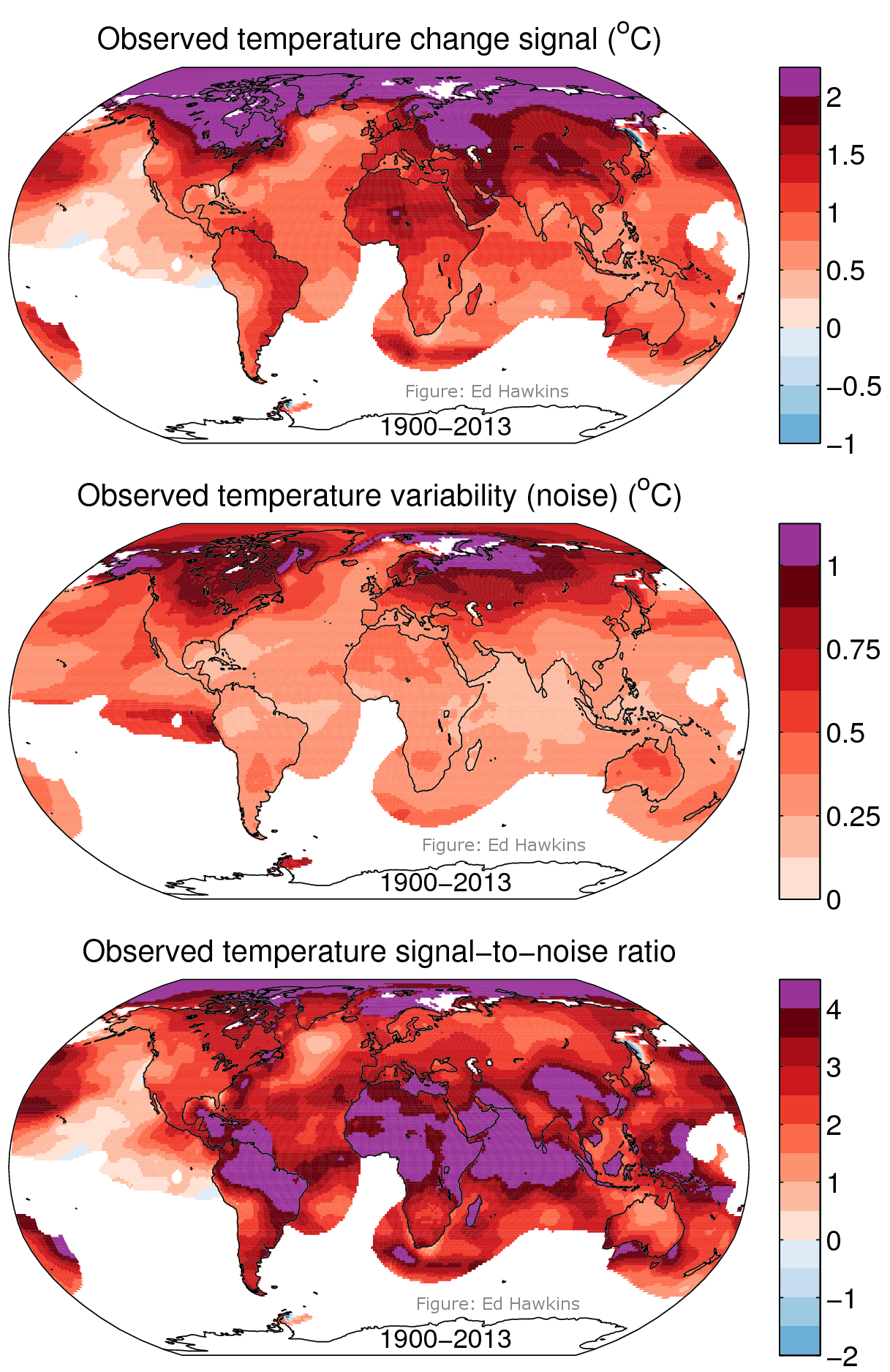
Using annual mean temperatures from the Berkeley Earth Temperature dataset, Figure 1 shows a simple estimate of the signal of temperature increase since 1900 (top panel), the amplitude of internal climate variability (or noise) (middle) and the signal-to-noise ratio (bottom). The methods are described at the bottom of the post.
The largest absolute temperature increases are in the Arctic, but the variability there is also large. The tropical regions have a smaller temperature increase, but the variability is small. Together, the ratio shows that the tropical regions have the largest signal relative to the size of climate variability. When considering temperature changes in this way, it is actually the tropical regions that are experiencing the largest impacts of climate change.
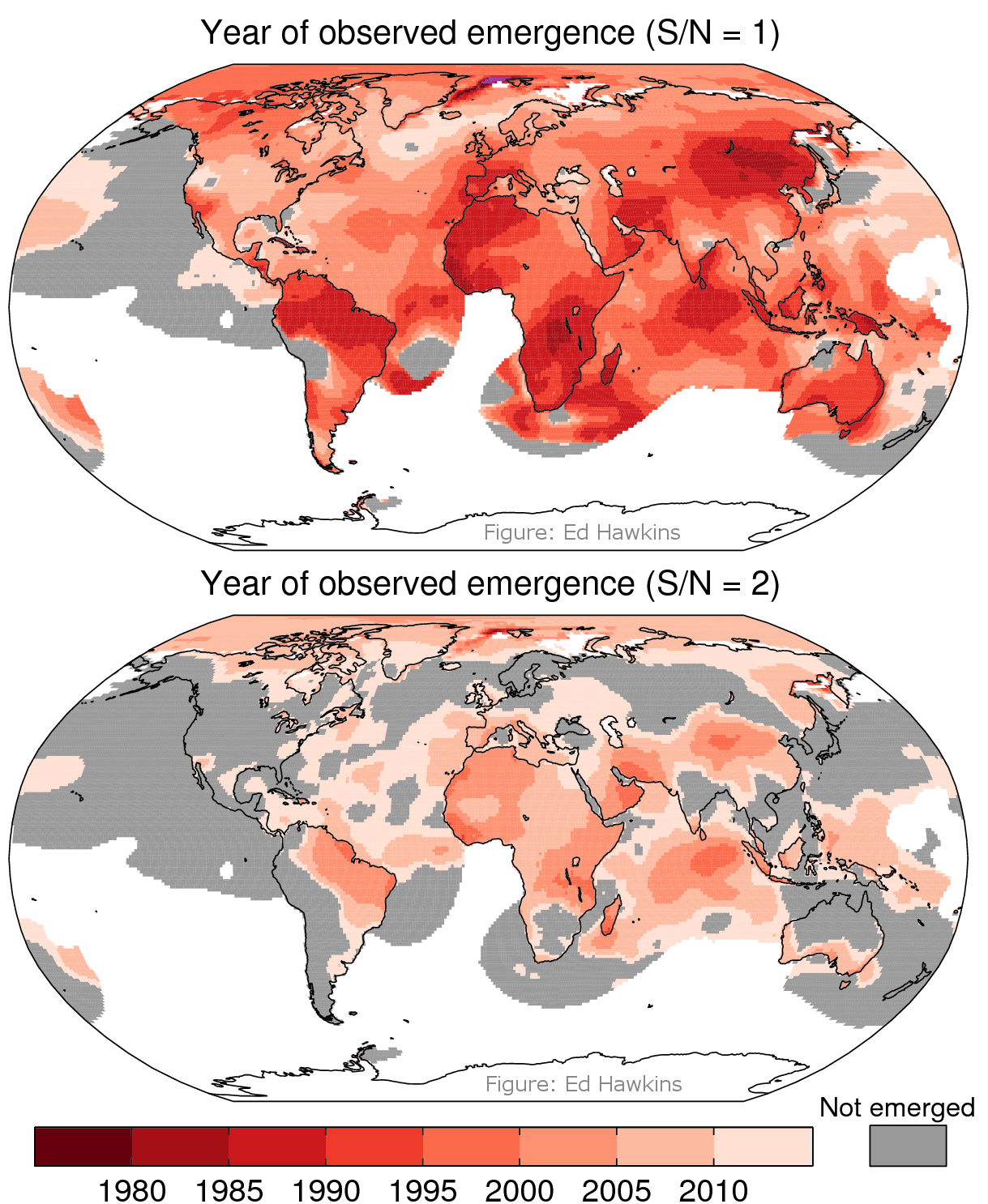
A related question is considering when the signal-to-noise ratio (S/N) crossed a particular threshold (such as 1 or 2) – this is called the ‘time of emergence’. Figure 2 shows that the earliest emergence times (in the 1980s) are found in the tropical regions. Most of the Arctic emerged in the 1990s and the extratropical regions have emerged later (2000s), or have not emerged yet. The dates are later for larger S/N values.
However, note especially that there is considerable spatial variability in the year of emergence – nearby regions can emerge more than a decade apart. These differences are due to the particular timing of the random climate fluctuations which causes some regions to apparently emerge slightly earlier, and some slightly later.
On a different ‘Earth’, the signal and amplitude of noise would be similar, but the experienced climate fluctuations would be different – the regions which emerge earliest would still be in the tropics, but each region would seem to emerge at a slightly different time. This will be important for the next post in this series.
Note that this is just a simple illustration of a well known finding – e.g. see Mahlstein et al. (2012), who did a more complex analysis. The IPCC AR5 Summary for Policymakers also noted that: “Relative to natural internal variability, near-term increases in seasonal mean and annual mean temperatures are expected to be larger in the tropics and subtropics than in mid-latitudes (high confidence)”.
Methods:
1. Fit a quartic polynomial to temperatures at each grid point over the entire period with continuous annual temperatures (smooth fit).
2. Difference in the smoothed fit values between 1900 and 2013 defines the signal.
3. Standard deviation of residuals from smooth fit defines the noise.
4. Signal-to-noise is simply the ratio of signal and noise.
5. The year of emergence is the first year when various S/N thresholds are permanently crossed.
6. Note that this is a simplified estimate of the signal-to-noise, with the caveat that it relies on the smooth fit to define the signal. This probably implies a slight underestimate of the variability and slight overestimate of the S/N.
What periods are the variabilities measured for? Daily, monthly or annual?
Thanks Ed – this is all done with annual mean temperatures – have tweaked the text to say this.
cheers,
Ed.
This seems like a rather arbitrary definition of ‘signal’ and ‘noise’.
Why a quartic polynomial? If you used a higher degree polynomial you’d get a better fit and therefore smaller ‘noise’ and faster ’emergence’.
Also, from a maths point of view polynomial fitting is not very popular. Why not use, say, a straight line plus 2 or 3 sin waves?
Hi Paul,
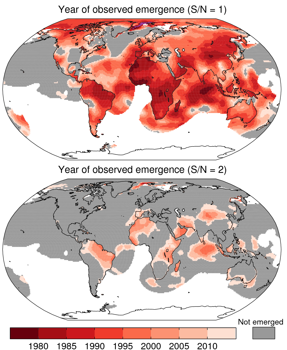
I agree – but to some extent, any choice of ‘signal’ is rather arbitrary – e.g. how many sine waves etc. And, yes, higher order polynomials would give earlier emergence times. This post is illustrating a few points – the relevance of which will become apparent at 6pm on Weds 2nd July….
This is the emergence year using a 2nd order polynomial for example, which has earlier emergence in some regions, and later emergence in others:
cheers,
Ed.
Very clear, and great graphics, thanks Ed.
I agree that Paul has a point–there’s a sensitivity to how S and N are defined. What do you get if you just let the trend be a straight line and the noise everything else?
Thanks Jim – yes, I agree – see reply to Paul above where I’ve used a quadratic to define the signal instead.
cheers,
Ed.
Great–thanks Ed. Pretty highly robust result I would have to conclude: I don’t see major differences between the two.
Jim – wonder whether you saw these 3 tweets – something you may be interested in?
https://twitter.com/ed_hawkins/status/483594496660504578
https://twitter.com/ed_hawkins/status/483595047116734464
https://twitter.com/ed_hawkins/status/483594679674732544
cheers,
Ed.
Thanks Ed–I’d missed ’em somehow.
A nice way to present the data. A friend of mine did something similar for precip:
D. Maraun. When will trends in European mean and heavy daily precipitation emerge? Env. Res. Lett. 8 014004, doi:10.1088/1748-9326/8/1/014004, 2013.
Just out of interest, how does what you’ve done here differ from an attribution study? Is it essentially the same, or is there some fundamental difference between an attribution study and a time of emergence study?
Thanks And Then There’s Physics – here, there is no formal attribution. We assume that there is a forced signal, which is somewhat arbitrarily defined as a smooth trend fit to the observations. But, this says nothing about the causes of the trend. It would be possible to use more complex models to define the signal – such as EBMs and GCMs – instead, and do a more formal test.
But, the aim of this post is to highlight that the tropics are experiencing changes outside what they have experienced before, and so the impacts there might be seen earlier. This is a way of considering climate changes differently from just absolute changes in temperature.
cheers,
Ed.
Ed,
Thanks. That makes sense.
Yes, that is very useful and I don’t think I’ve really seen this illustrated this way before.